Sage Journals: Discover world-class research

Abstract

There are two difficulties in the remaining useful life prediction of rolling bearings. First, the vibration signals are always interfered by noise signals. Second, some of the extracted features include useless information which may decrease the prediction accuracy. In order to solve the problems above, corresponding methods are employed in this article. First, adaptive sparsest narrow-band decomposition is utilized for extracting the degradation information from noise. Compared with the commonly used empirical mode decomposition method, problems including mode mixture and boundary effect caused by the calculation of extremas is not required. Second, locality-preserving projection is applied for merging the meaningful information from the original data and reduces the dimension of features. Based on adaptive sparsest narrow-band decomposition and locality preserving projection, a novel approach is employed for the remaining useful life prediction. The prediction procedure is as follows. First, the signals are analyzed by adaptive sparsest narrow-band decomposition and the feature vectors are constructed. Afterwards, the features are fused by locality preserving projection to merge useful information from the features. Least squares support vector machine is applied for the remaining useful life prediction in the end. The analysis results indicate that the proposed approach is reliable for rolling bearing remaining useful life prediction.

Keywords

Adaptive sparsest narrow-band decomposition locality preserving projections least squares support vector machines rolling bearing remaining useful life

Introduction

As rolling bearing fault has become one of the most frequently happened reason in the failure of mechanical systems, research on the prediction of remaining useful life (RUL) has become a hotspot in case-dependent maintenance.^1–11 The RUL prognostic methods can be divided into model-based approaches^1–4 and data-based approaches.^5–9 In model-based approaches, the forecasting problem is solved by mathematical equations. Based on the propagation theory of rolling bearing, an approach for operating state prognosis of rolling bearings was proposed by Marble and Morton.¹ Liao et al.² introduced a RUL forecasting approach using logistic or hazard regression models. A proportional hazard model was introduced by Tian and Liao³ for the RUL prediction. Model-based approaches can predict the RUL prediction accurately if properly applied. The dynamic procedure and fault spread of mechanical systems are complicated. Thus, it is very hard to construct the model.

In data-based approaches, the data sets obtained from various conditions and appropriate signal processing methods are utilized. Data-based approaches are more appropriate for complicated situations as the equations and the physical laws of rolling bearing do not have to be considered. Gebraeel et al.⁴ developed an approach for the RUL prediction of bearings using neural network. Maio et al.⁵ developed an approach using relevance vector machine for the estimation of RUL. Ali et al.⁶ introduced an approach by applying Weibull distribution.

In the data-driven methods, empirical mode decomposition (EMD) is pervasively used to reduce the fluctuation for feature extraction on the degradation trend of bearings.^7–9 As it has shown a better performance in analyzing simulation and experimental signals than EMD,¹² adaptive sparsest narrow-band decomposition (ASNBD) algorithm is introduced to extract feature.

The ASNBD algorithm was proposed by combining the theory of matching pursuit (MP)^13–15 and EMD.^16–19 It has shown a good performance in analyzing mechanical vibration signals. In ASNBD, the sparsest decomposition of a complex signal is gained by limiting the components as local narrow-band (LNB).²⁰ A designed filter must be optimized in ASNBD at first. The optimization objective function is set to be a differential operator²⁰ to constrain the components as LNB signals. The complex signals are smoothed by applying the optimal filter to obtain LNB component.

The decomposition results are with physical meaning in ASNBD, which is similar to EMD. Nevertheless, in the decomposition process, optimization problems are solved in ASNBD to replace the interpolation function in EMD. Therefore, the drawbacks including mode mixture and boundary effect in EMD which are caused by the application of interpolation function are alleviated in ASNBD. The similarity between MP and ASNBD is that the sparsest decomposition results are both obtained by solving optimization problems. However, a redundant dictionary should be constructed in MP before it is applied, which is not necessary in ASNBD. So that ASNBD shows a better performance in adaptivity. Otherwise, the analysis results of ASNBD possess more explicit meaning.

It is noted that not all the information in the extracted features are beneficial to the rolling bearing RUL prediction. Therefore, appropriate techniques should be utilized to merge the useful information from the extracted features and reduce the dimension of features. Many advanced algorithms containing principal component analysis (PCA),²¹ linear discriminant analysis,²² locally linear embedding,²³ and kernel PCA²⁴ have been proposed to achieve that goal. Locality preserving projections (LPPs)²⁵ was developed by He et al.²⁵ It can generate linear projective map that possesses the intrinsic information of the signals in a lower dimensional space. As LPP has been proven to be beneficial for mechanical vibration signal analysis in many articles,^26–28 it is applied to fuse the features obtained from the experimental data sets in the proposed method.

The process of the RUL prediction is as follows. First, each collected data is decomposed by ASNBD, and some statistical parameters of each signal are calculated. Afterwards, the features are fused by applying LPP, and least squares support vector machine (LS-SVM)^10,11 is applied for RUL prediction.

The remaining contents are as follows. The relevant approaches and the process of the proposed approach are given out in section “Methodology.” The validity of the proposed approach is tested in section “Experimental analysis.” In section “Conclusion,” the conclusions and discussions are given.

Methodology

ASNBD method

Mechanical vibration model

Impulses are produced while a rolling bearing strikes with another one.²⁹ The collected vibration data are periodically modulated by the impulses. The vibration model is as follows³⁰

x (t) = \sum_{- \infty}^{+ \infty} h (t - iT) q (iT) + n (t)

(1)

where $h (t)$ denotes the generated impulse, $x (t)$ is the collected signal, $q (t)$ represents the periodic modulation, $n (t)$ is the noise interference, and $i$ denotes the ith impulse.

The $h (t)$ is comprised of a number of cosine signals due to Fourier transform (FT). Meanwhile, the frequencies modulating the collected vibration signal is narrowband. Thus, the mechanical model of a vibration signal can be defined

x (t) = s (t) + n (t)

(2)

where $s (t) = \sum_{i = - \infty}^{+ \infty} a_{i} (t) g_{i} (ω t + ϕ (t))$ denotes the assembly of modulation signals.

From the model in equation (2), it can be found that a vibration signal has two parts: the useful part which contains the fault information and the useless part which contains the noise information. Thusly, the process of extracting useful information from the vibration signal can be considered as the process of separating the periodic modulation signal $s (t)$ from noise signal $n (t)$ . For convenience, the ith component $a_{i} (t) g_{i} (ω t + ϕ (t))$ is defined to be LNB signal. More details of the LNB signals will be introduced in the following.

Intrinsic narrow-band component

A narrow-band signal is commonly expressed to be $A (t) \cos (ω t + ϕ (t))$ , $ω$ is much bigger than the maximum frequency of $A (t)$ , $A (t)$ is narrowband, $ϕ (t)$ is slow-varying.

For a signal, if any neighborhood interval is close to be narrow-band, then it is an LNB signal.²⁰ Moreover, if the decomposed components satisfy the definition of LNB signal, they are defined as intrinsic narrowband components (INBCs).

Singular local linear operator

For a singular linear operator, if any neighborhood $B_{t}$ satisfy the following condition

T (S) (t) = T (S |_{B_{t}}) (t)

(3)

where $S |_{B_{t}} = S (t)$ or $S |_{B_{t}} = 0$ , and then T is a singular local linear operator.²⁰

The singular local linear operator T introduced by Peng et al. is as follows

T = {(\frac{1}{ω^{2}} \frac{d^{2}}{d t^{2}} + 1)}^{2}

(4)

It can be easily inferred that for an LNB $s (t) = A (t) \cos (ω t + φ (t))$ . $ω$ is much bigger than the maximum frequency of $A (t)$ , we have $((1 / ω^{2}) (d^{2} / d t^{2}) + 1)^{2} s (t) = 0$ . Thus, INBCs can be obtained by minimizing $T (s) (t)$ so that the components are constrained to be LNB signals.

ASNBD scheme

ASNBD searches for the sparsest decomposition by solving optimization problems in ASNBD. Assume there is a complex signal $x (n), n = 1, 2, 3, \dots, N$ . The iterative procedure is as follows:

1. Make $r_{0} (n) = x (n)$ and $i = 1$ ;

2. $P_{1}$ is presented as follows

\begin{matrix} P_{1} : Minimize ‖ T (INB C_{i} (n)) ‖_{2}^{2} \\ + λ ‖ D (r_{i - 1} (n) - INB C_{i} (n)) ‖_{2}^{2} \end{matrix}

(5)

The differential operator T is defined in equation (4), which is applied to constrain $INB C_{i} (n)$ to be LNB. D is a first-order differentiation operator used for regulating the residual. $λ$ is a weight factor. Besides, experimental results show that $λ$ can be set as 20 for analyzing the whole-life vibration data sets:

3. Set $r_{i} (n) = r_{i - 1} (n) - INB C_{i} (n)$ to update the residual;

4. Stop the iteration process if $‖ r_{i} (n) ‖_{2}^{2} < ε$ . Otherwise return to step 2, set $i = i + 1$ .

In P₁ of equation (5), all the data points in $INB C_{i} (n)$ should be optimized. There are N parameters to be optimized in every iteration process. Thus, massive calculation is needed on this occasion. To reduce the calculated amount, the following algorithm is proposed:

1. Obtain the fast Fourier transformation of the original signal $r_{i} (n)$ and denote as ${\hat{r}}_{i} (k)$ ;

2. A nonlinear filter $χ (k | η)$ $(η = [ω, ω_{b}, ω_{c}])$ is designed as equation (6) (see also Figure 1)

χ (k | η) = {\begin{matrix} \sin ω [\frac{k - ω_{c} + ω_{b} + π}{(2 ω)}], & \frac{ω_{c} - ω_{b} - π}{(2 ω)} \leq k < ω_{c} - ω_{b} \\ 1, & ω_{c} - ω_{b} \leq k \leq ω_{c} + ω_{b} \\ \cos ω (k - ω_{c} - ω_{b}), & ω_{c} + ω_{b} < k \leq \frac{ω_{c} + ω_{b} + π}{(2 ω)} \\ 0, & else \end{matrix}

(6)

3. Solve $P_{2}$ presented below

P_{2} : Minimize ‖ T [INB C_{i} (n)] ‖_{2}^{2} + λ ‖ D [r_{i} (n) - INB C_{i} (n)] ‖_{2}^{2}

(7)

Figure 1.

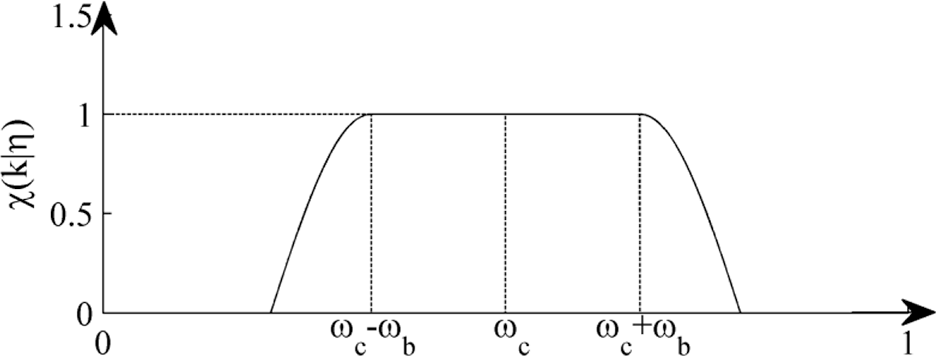
The filter given in equation (6).

The parameter vector $η$ is optimized by solving $P_{2}$ . The optimal $η$ is represented as $η_{0}$ :

4. Set $INB C_{i} (n)$ to be the Fourier inversion of $χ (k | η_{0}) {\hat{r}}_{i} (k)$ .

Figure 2 illustrates the ASNBD procedure. The optimization problem P₁ in the original algorithm is replaced with the optimization P₂ of the parameter vector $η$ . Therefore, the optimization of the N parameters in the original algorithm is changed into optimizing the parameter vector $η$ to reduce the calculated amount. The unconstrained nonlinear optimization problem $P_{2}$ is solved by applying genetic algorithm (GA) method.

Figure 2.

The flow chart of ASNBD.

Cyclostationary signal analysis

As vibration signals of rolling bearings are cyclostationary signals in essence.³¹ To verify the validity of ASNBD method, two cyclostationary signals are applied in this section. The signals are handled by both EMD and ASNBD for the purpose of comparison. First, a cyclostationary signal $x (t)$ is considered as follows

{\begin{matrix} x_{1} (t) = [\cos (8 π t) + 1] \cos [120 π t + \sin (8 π t)] \\ x (t) = x_{1} (t) + n_{1} (t) \\ t = 0 : 1 / 2048 : 1 \end{matrix}

(8)

where $x (t)$ contains a multiplied signal $x_{1} (t)$ and a random noise signal $n_{1} (t)$ . The amplitude and the mean of $n_{1} (t)$ is set to be 0.5 and 0. The waveforms of $x (t)$ are given in Figure 3.

Figure 3.

The time-domain waveforms of simulation signal x(t) in equation (8) and its components.

The decomposed components of $x (t)$ using EMD and ASNBD are shown in Figures 4 and 5, respectively. The two components are obtained directly by ASNBD and are similar to the true values, but the intrinsic mode function (IMF₂) obtained by EMD has obvious mixed modes and a false component IMF₂ appears. Then Hilbert transform (HT)¹⁹ is utilized to obtain instantaneous amplitudes (IAs) and instantaneous frequencies (IFs) of the components corresponding to the real component $x_{1} (t)$ (INBC₁ and IMF₂). The IAs of INBC₁ and IMF₂ and their absolute errors between actual values are given in Figure 6(a) and (b). The IFs and their absolute errors between actual values are given in Figure 6(c) and (d). The HT results of IMF₂ derived by EMD method are severely influenced by mode mixing. The fluctuations and the absolute errors are very obvious. Thusly, it can be concluded that the IAs and the IFs of the INBC₁ derived by ASNBD are superior in absolute errors and fluctuation.

Figure 4.

The decomposition results generated by ASNBD.

Figure 5.

The decomposition results generated by EMD.

Figure 6.

The IAs and IFs and their absolute errors between real values: (a) the IAs of INBC₁ and IMF₂, (b) the absolute errors of the IAs of INBC₁ and IMF₂, (c) the IFs of INBC₁ and IMF₂, and (d) the absolute errors of the IFs of INBC₁ and IMF₂.

For further comparison, the parameters such as energy error $E_{i}$ , index of orthogonality $IO$ , and correlation coefficient $r_{i}$ are calculated

E_{i} = \frac{\sum_{n = 1}^{N} {(S_{i} (n) - I_{i} (n))}^{2}}{\sum_{n = 1}^{N} I_{i} {(n)}^{2}}

(9)

IO = \sum_{n = 1}^{N} \sum_{i = 1}^{M} \sum_{j = 1}^{M} \frac{S_{i} (n) S_{j} (n)}{x^{2} (n)}

(10)

r_{i} = \frac{\sum_{n = 1}^{N} (S_{i} (n) - {\bar{S}}_{i}) (I_{i} (n) - {\bar{I}}_{i})}{\sqrt{\sum_{n = 1}^{N} {(S_{i} (n) - {\bar{S}}_{i})}^{2} \sum_{n = 1}^{N} {(I_{i} (n) - {\bar{I}}_{i})}^{2}}}

(11)

In equations (9)–(11), $S_{i} (n)$ and $I_{i} (n)$ are the obtained and actual values, and ${\bar{S}}_{i}$ and ${\bar{I}}_{i}$ are the means of the obtained and actual values.

$E_{i}$ , $r_{i}$ are used to verify the precision between the derived signals and the real values. $IO$ is applied to evaluate the orthogonality of ASNBD.

The calculated parameters in Table 1 show that INBC₁ is closer to the real component $x_{1} (t)$ than EMD. The energy errors of INBC₁ are much smaller than IMF₂. Thus, the results obtained by ASNBD are more accurate than EMD. Meanwhile, the index of orthogonality (IO) of ASNBD indicates better orthogonality.

Table 1.

Evaluating parameters of the components of x(t) generated by ASNBD and EMD.

Component	r ₁	E ₁	IO
INBC ₁	0.9817	0.0363	0.0021
IMF ₂	0.6795	0.7001	0.3031

ASNBD: adaptive sparsest narrow-band decomposition; EMD: empirical mode decomposition; INBC: intrinsic narrowband components; IMF: intrinsic mode function; IO: index of orthogonality.

Furthermore, a more complicated cyclostationary signal is considered

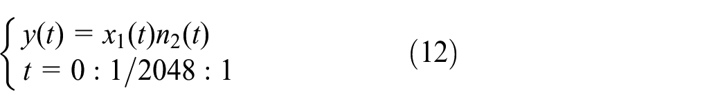
{\begin{matrix} y (t) = x_{1} (t) n_{2} (t) \\ t = 0 : 1 / 2048 : 1 \end{matrix}

(12)

In the cyclostationary signal $y (t)$ , a random noise signal $n_{2} (t)$ of which the amplitude is 0.2 and the mean is 1 is applied to modulate $x_{1} (t)$ in equation (8). The $y (t)$ is illustrated in Figure 7, the decomposed components are given in Figures 8 and 9. The INBC₁ in Figure 8 is much more appropriate to $x_{1} (t)$ compared with IMF₃ in Figure 9, which suggests that the component obtained by ASNBD is more accurate. The IA, the absolute error of IA, the IF, and the absolute of IF which are calculated from INBC₁ and IMF₃ are given in Figure 10(a)–(d). Although the IA and IF of INBC₁ have slight fluctuation owe to the modulation of the noise signal, it is still much more appropriate to the real values compared with IMF₃. The statistical parameters in Table 2 also indicate that ASNBD precedes in both the precision and orthogonality.

Figure 7.

The time-domain waveforms of simulation signal y(t) in equation (12) and its components.

Figure 8.

The decomposition results generated by ASNBD.

Figure 9.

The decomposition results generated by EMD.

Figure 10.

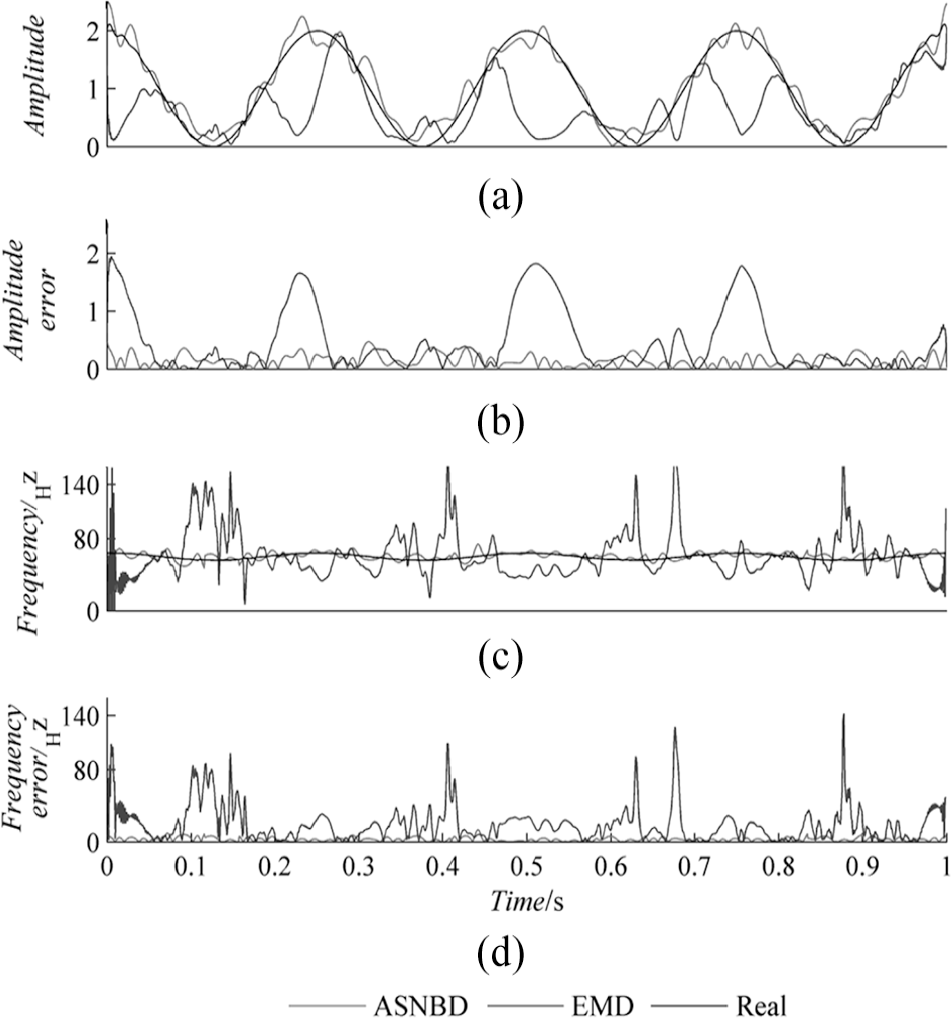
IAs and IFs and their absolute errors between real values: (a) the IAs of INBC₁ and IMF₃, (b) the absolute errors of the IAs of INBC₁ and IMF₃, (c) the IFs of INBC₁ and IMF₃, and (d) the absolute errors of the IFs of INBC₁ and IMF₃.

Table 2.

Evaluating parameters of the components of y(t) generated by ASNBD and EMD.

Component	r ₁	E ₁	IO
INBC ₁	0.9047	0.2003	0.0051
IMF ₃	0.6696	0.7620	0.5031

ASNBD: adaptive sparsest narrow-band decomposition; EMD: empirical mode decomposition; INBC: intrinsic narrowband components; IMF: intrinsic mode function; IO: index of orthogonality.

It can be concluded that when $x_{1} (t)$ is mixed or modulated by a random noise signal, ASNBD precedes EMD in both orthogonality and accuracy. That is to say, while applied to cyclostationary signals such as $x (t)$ and $y (t)$ , ASNBD is more stable for noise interference than EMD.

Statistical parameters

After the vibration data sets are decomposed by ASNBD, statistical parameters should be calculated to extract the features. Table 3 shows some common features. For the convenience of calculating, the parameters are all normalized. More details about the statistical parameters can be found in Zeng et al.³² As the generated components with high frequency are usually generated first and bearing fault information often exists in the high-frequency bands, the first several INBCs are selected in practical applications.³²

Table 3.

Statistical parameters.

Frequency domain statistical parameters		Time domain statistical parameters
Mean: $F_{1} = \frac{1}{N} \sum_{n = 1}^{N} x (n)$	Skewness: $F_{7} = \frac{1}{N - 1} \sum_{n - 1}^{N} {(\frac{x (n) - F_{1}}{F_{6}})}^{3}$	Spectral amplitude mean: $F_{13} = \frac{1}{M} \sum_{k = 1}^{M} s (k)$	Spectral root 4/2-moment ratio: $F_{19} = \sqrt{\frac{\sum_{k = 1}^{M} f^{4} (k) s (k)}{\sum_{k = 1}^{M} f^{2} (k) s (k)}}$
Root mean square: $F_{2} = \sqrt{\frac{1}{N} \sum_{n = 1}^{N} x^{2} (n)}$	Kurtosis: $F_{8} = \frac{1}{N - 1} \sum_{n - 1}^{N} {(\frac{x (n) - F_{1}}{F_{6}})}^{4}$	Spectral amplitude standard deviation: $F_{14} = \sqrt{\frac{1}{M - 1} \sum_{k = 1}^{M} {(s (k) - F_{13})}^{2}}$	Spectral standard deviation frequency: $F_{20} = \sqrt{\frac{\sum_{k = 1}^{M} {(f (k) - F_{17})}^{2} s (k)}{\sum_{k = 1}^{M} s (k)}}$
Square root amplitude: $F_{3} = {(\frac{1}{N} \sum_{n = 1}^{N} \sqrt{\| x (n) \|})}^{2}$	Crest factor: $F_{9} = \frac{F_{5}}{F_{2}}$	Spectral amplitude skewness: $F_{15} = \frac{1}{M - 1} \sum_{k = 1}^{M} {(\frac{s (k) - F_{13}}{F_{14}})}^{3}$	Spectral frequency skewness: $F_{21} = \sum_{k = 1}^{M} \frac{{(\frac{f (k) - F_{17}}{F_{20}})}^{3} s (k)}{\sum_{j = 1}^{M} s (j)}$
Mean amplitude: $F_{4} = \frac{1}{N} \sum_{n = 1}^{N} \| x (n) \|$	Clearance factor: $F_{10} = \frac{F_{5}}{F_{3}}$	Spectral amplitude kurtosis: $F_{16} = \frac{1}{M - 1} \sum_{k = 1}^{M} {(\frac{s (k) - F_{13}}{F_{14}})}^{4}$	Spectral frequency kurtosis: $F_{21} = \sum_{k = 1}^{M} \frac{{(\frac{f (k) - F_{17}}{F_{20}})}^{4} s (k)}{\sum_{j = 1}^{M} s (j)}$
Maximum peak: $F_{5} = \frac{1}{2} (max (x (n)) - min (x (n)))$	Shape factor: $F_{11} = \frac{F_{2}}{F_{4}}$	Spectral gravity frequency: $F_{17} = \frac{\sum_{k = 1}^{M} f (k) s (k)}{\sum_{k = 1}^{M} s (k)}$
Standard deviation: $F_{6} = \sqrt{\frac{1}{N - 1} \sum_{n = 1}^{N} {(x (n) - F_{1})}^{2}}$	Crest factor: $F_{12} = \frac{F_{5}}{F_{4}}$	Spectral root mean square frequency: $F_{18} = \sqrt{\frac{\sum_{k = 1}^{M} f^{2} (k) s (k)}{\sum_{k = 1}^{M} s (k)}}$

LPP method

After the statistical parameters are obtained from the vibration signals of rolling bearings, an M dimensional feature vector can be constructed. However, the generated feature vector always includes superfluous information and is high dimensional. Thus, appropriate technique should be applied to extract effective information and decrease the dimension of the features. The PCA is the most common method for the dimensionality reduction in the RUL prediction.^21,33 The PCA is meant for gaining the global information of Euclidean space and short of the ability of preserving the global structure.^21,33 To avoid that disadvantage, LPP method, which can discover local information of the collected data, is applied in this article.^26–28

The LPP preserves a local structure by extracting a linear approximation of the original feature. Assume $F = {f_{1}, f_{2}, \dots, f_{N_{i}}}$ is the feature data sets. J, N_i are the numbers of the features and the samples. LPP searches a mapping matrix to fuse the features into lower dimensional data sets $F^{'} = {f'_{1}, f'_{2}, \dots, f'_{N_{i}}}$ , where $J' (J' \times J)$ is the dimension of the fused feature $F'$ . In order to choose such a map, the objective function is defined as follows^26–28

min \sum_{i, j = 1}^{N_{i}} {‖ f_{i} - f_{j} ‖}^{2} S_{i, j}

(13)

The weight S is gained by the nearest-neighbor graph and incurs a penalty when the neighboring points $f_{i}$ and $f_{j}$ are very far apart. The definition of S is as follows

S_{i, j} = {\begin{matrix} \exp (\frac{- {‖ f_{i} - f_{j} ‖}^{2}}{(2 σ^{2})}), f_{i} or f_{j} is between the k nearest neighbors \\ of f_{j} or f_{i}, respectively \\ 0 \end{matrix}

(14)

where k expresses the “locality” of the local neighborhood and $σ$ represents the main kernel. The object function is minimized for making sure $f_{j}$ and $f_{i}$ are near, hence $f'_{j}$ and $f'_{i}$ are also near. Thus, the local information in the original feature data sets F is preserved. Assume $f'_{i} = a^{T} f_{i}$ , then the optimization problem in equation (13) is changed as follows

\begin{matrix} J_{l} (a) & = \frac{1}{2} \sum_{i, j = 1}^{N_{i}} {‖ {f'}_{i} - {f'}_{j} ‖}^{2} S_{i, j} = \frac{1}{2} \sum_{i, j = 1}^{N_{i}} {‖ a^{T} f_{i} - a^{T} f_{j} ‖}^{2} S_{i, j} \\ = a^{T} F (D - S) F^{T} a = a^{T} FL F^{T} a \end{matrix}

(15)

where D $(D_{ii} = \sum_{j} S_{i, j})$ is a defined matrix. $L = D - S$ is a Laplacian matrix. A bigger $D_{ii}$ means a more significant $f'_{i}$ . Then, a constrain is imposed by LPP as follows

F'^{T} DF' = 1 \Rightarrow aFD F^{T} a = 1

(16)

The optimization problem is as follows

min_{a} aFL F^{T} a subject to aFD F^{T} a = 1

(17)

The constricted optimization objective operator can be changed into a generalized eigenvalue problem by applying Lagrange multiplier approach. Thus, the following transformation matrix is obtained

FL F^{T} a = λ FD F^{T} a

(18)

where $λ$ represents the eigenvalue. The reduction of the dimension is as follows

F' = A^{T} FA = [a_{1}, a_{2}, \dots, a_{l}]^{T}

(19)

where A is a $J \times J'$ matrix and a fused vector $F'$ is obtained after the original inputted vector $F$ is projected. The local variation information is preserved by $F'$ as well as the dimension is reduced. Thus, LPP is capable of seeking the optimized linear local structure in the matrix. Meanwhile, the local preserving property makes LPP to be suitable for noise and isolated values.

PCA is utilized for extracting the subspace to maximize variance, thus it can preserve the global structure. Nevertheless, the information in the local structure of real-world data sets such as mechanical vibration signals is more important. Besides, LPP has been proved to be suitable for processing the vibration signals of rolling bearings. Meanwhile, comparisons has been made between LPP and PCA by applying vibration signals, and the results has shown that PCA is superior in extracting useful information from the original feature vectors.^26–28 Thusly, LPP method, which can preserve the local information of data sets, is applied in the propose method for the dimensionality reduction.

Least squares support vector machine

The LS-SVM is the modified algorithm of SVM, which is proposed for dealing with nonlinear and high-dimensional occasions. The LS-SVM procedure is as follows.^10,11

For a data set $(x_{i}, y_{i}) i = 1, 2, 3, \dots, n$ . The LS-SVM representation is as follows

f (x_{i}) = w^{T} φ (x_{i}) + b

(20)

where w is the weight value; b is the bias value. The optimization problem J is constructed as follows

J (w, e_{i}) = \frac{1}{2} ‖ w^{2} ‖ + \frac{1}{2} C \sum_{i = 1}^{N} e_{i}^{2}

(21)

y_{i} = w^{T} φ (x_{i}) + b + e_{i}

(22)

Equation (21) is the object function and equation (22) is the constraint, C is a regulation value, and $e_{i}$ is the degeneration error. Lagrange multipliers is applied for solving the problem as follows

L (ω, a_{i}, b, e_{i}) = J (ω, e_{i}) + \sum_{i = 1}^{N} a_{i} [y_{i} - ω^{T} φ (x_{i}) - b - e_{i}]

(23)

Obtain the first-order differentiation of equation (23)

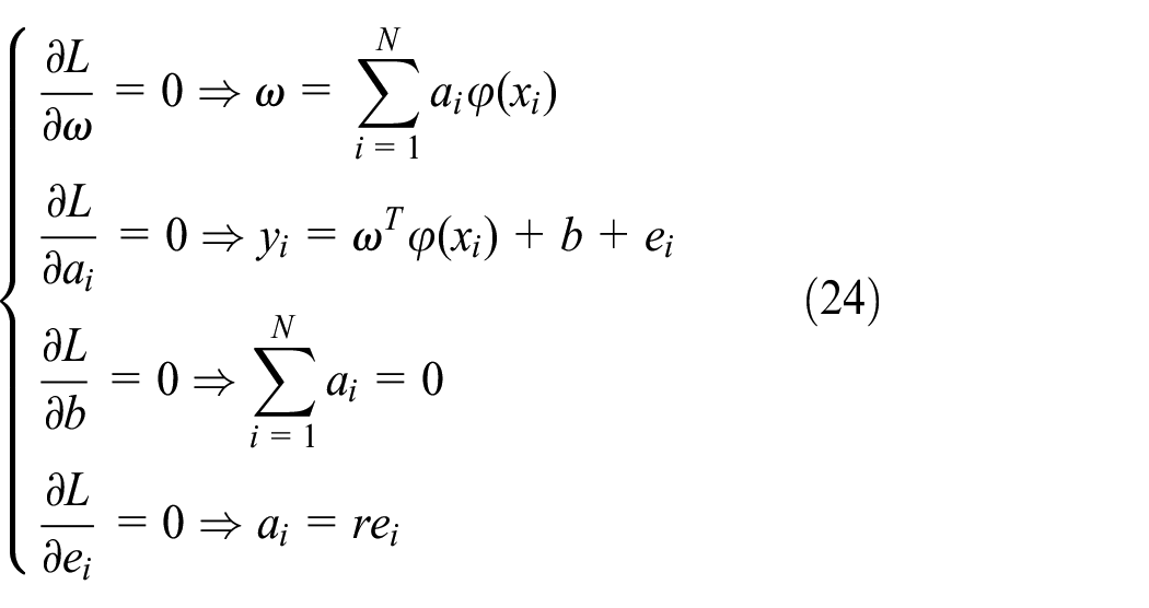
{\begin{matrix} \frac{\partial L}{\partial ω} = 0 \Rightarrow ω = \sum_{i = 1}^{N} a_{i} φ (x_{i}) \\ \frac{\partial L}{\partial a_{i}} = 0 \Rightarrow y_{i} = ω^{T} φ (x_{i}) + b + e_{i} \\ \frac{\partial L}{\partial b} = 0 \Rightarrow \sum_{i = 1}^{N} a_{i} = 0 \\ \frac{\partial L}{\partial e_{i}} = 0 \Rightarrow a_{i} = r e_{i} \end{matrix}

(24)

After the parameters $ω$ and $e_{i}$ are removed, the formula can be obtained as follows

[\begin{matrix} 0 & {(l_{n})}^{T} \\ l_{n} & Ω + I / r \end{matrix}] [\begin{matrix} b \\ a \end{matrix}] = [\begin{matrix} 0 \\ y \end{matrix}]

(25)

where $l_{n} = (1, 1, 1, \dots, 1)^{T}$ , $a = (a, a_{1}, \dots, a_{n})$ , $y = (y_{1}, y_{2}, \dots, y_{n})$ , $Ω_{ij} = φ (x_{i})^{T} φ (x_{j})$ , and I is a unitary matrix. The LS-SVM model is finally gained as follows

\hat{y} (x) = \sum_{i = 1}^{N} a_{i} K (x, x_{i}) + b

(26)

The proposed method

An approach for RUL prognosis is introduced based on ASNBD and LPP. The flow chart is illustrated as Figure 11. The process of the approach is as follows:

The collected RUL signals are separated using ASNBD; the M first extracted INBCs are employed.

The statistical features of the INBCs are calculated. As the M first extracted INBCs are applied, the feature vectors’ number F is $(M + 1) \times 22$ .

The features are fused by LPP method to lower the dimension of the features and merge useful information. Then the fused feature is normalized.

The LS-SVM classifier is applied for testing and training; output the predicted RUL results of rolling bearing.

Figure 11.

The flow chart of the method proposed in section “Least squares support vector machine.”

Experimental analysis

The collected experimental signals are from the Center for Intelligent Maintenance Systems (IMS) of Cincinnati University.^34–36 The type of the used bearings is Rexnord ZA-2115. In every row of the bearings, there are 16 rollers. The PCB 353B33 ICP accelerometers with high sensitivity are set on the bearing house. The test rig is shown in Figure 12. Four bearings are applied for testing in the experiment. The radial load is set to 6000 lbs and the rotation speed is set to 2000 r/min. The experiment lasted 35 days to obtain the whole life data of the bearings.

Figure 12.

Bearing test rig.

The signals are collected in 10 min. The sample frequency is set to 20 kHz. The experiment repeated three times, and all the four bearings are considered. Therefore, 12 data sets are collected in the whole experiment. However, only three bearings are failed in the test, which means corresponding three data sets can be seen as whole life data. The details of the three whole life experimental signals are illustrated in Table 4. For convenience, the signals are denoted as 1, 2, and 3, and the time domain curves are shown in Figure 13.

Table 4.

Information of the experimental data sets.

Data set	Test	Bearing	Break time (10 min)	Degradation type	Maximum magnitude (m/s²)
1	1	3	2156	Inner race	5
2	1	4	2156	Roller	4
3	2	1	984	Outer race	5

Figure 13.

Vibration signals of all the data sets: (a), (b), and (c) are the vibration signals of data set 1, 2, and 3, respectively.

First, LPP and PCA are applied to lower the dimension and extract useful information to testify the effectiveness of LPP. The eigenvectors of original data sets are all fused to be one-dimensional eigenvectors. The fused eigenvectors of the three data sets are illustrated in Figures 14 –16. The fused features obtained using the LPP show better similarity with time and the curves have obviously less fluctuation compared with PCA.

Figure 14.

Eigenvectors fused by LPP and PCA of data set 1: (a) and (b) are the fused eigenvectors generated by LPP and PCA, respectively.

Figure 15.

Eigenvectors fused by LPP and PCA of data set 2: (a) and (b) are the fused eigenvectors generated by LPP and PCA, respectively.

Figure 16.

Eigenvectors fused by LPP and PCA of data set 3: (a) and (b) are the fused eigenvectors generated by LPP and PCA, respectively.

Second, to verify the effectiveness of ASNBD, comparisons are made between the three methods including using the features of the original data sets, the INBCs obtained by ASNBD, and IMFs gained by EMD as the input of LPP. All the data sets are handled by ASNBD. Then the 22 statistical parameters are calculated. As only the first three INBCs are considered, there are 22 × 3 features of the INBCs obtained by ASNBD for testing the effectiveness of ASNBD. The features of the data sets and the first three components obtained using EMD are also calculated to construct the eigenvectors for comparison.

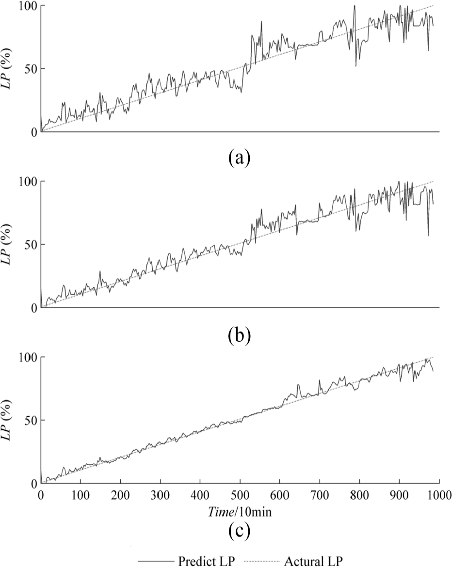
The LS-SVM is applied to fulfill the RUL prognosis process in the end. The 1/3 individual files with uniform interval are applied for testing and the others are used for training.Figures 17 –19 show the RUL prognosis results of the three data sets. Life percentage (LP) represents the degeneration degree of the rolling bearing. For example, if the total test time is 2156 min and current time is 200 min, the LP is calculated as 200/2156 (i.e. 9.276%). Figures 17 –19 show the predicted results of ASNBD are apparently more similar to the actual values. Otherwise, the fluctuations of the LP curves of ASNBD are smaller. To get a deeper insight about the proposed method, parameters generated by calculating the RUL prediction results are considered in Table 5. CA_i, r_i, and E_i are the mean classification accuracy, the correlation coefficient and the energy error between the RUL prediction results and the real values of the ith data set, respectively. E_i and r_i are defined in equations (9) and (10).

Figure 17.

The RUL prediction results of data set 2. (a), (b), and (c) are the predicted LP obtained by applying the original data sets, the decomposed components generated by EMD and ASNBD, respectively.

Figure 18.

The RUL prediction results of data set 2. (a), (b), and (c) are the predicted LP obtained by applying the original data sets, the decomposed components generated by EMD and ASNBD, respectively.

Figure 19.

The RUL prediction results of data set 3. (a), (b), and (c) are the predicted LP obtained by applying the original data sets, the decomposed components generated by EMD and ASNBD, respectively.

Table 5.

Evaluating parameters of the RUL prediction results.

Decomposition method	Data set 1			Data set 2			Data set 3
	r ₁	E ₁	CA ₁	r ₂	E ₂	CA ₂	r ₃	E ₃	CA ₃
Original data sets	0.9449	0.0270	0.8013	0.9253	0.0364	0.8322	0.9554	0.0219	0.5824
EMD	0.9801	0.0099	0.9437	0.9345	0.0322	0.9431	0.9698	0.0148	0.9613
ASNBD	0.9956	0.0022	0.9523	0.9845	0.0077	0.9944	0.9941	0.0030	0.9712

RUL: remaining useful life; CA: classification accuracy; EMD: empirical mode decomposition; ASNBD: adaptive sparsest narrow-band decomposition.

In Table 5, it can be inferred that the RUL prediction accuracies generated by utilizing ASNBD are superior. And the proposed method is performed better in the analysis of experimental data sets. Compared with EMD, ASNBD is more effective in extracting useful information from non-linear vibration data sets. Thusly, it can be inferred that the RUL prognosis approach based on ASNBD and LPP shows a superior performance in the RUL prediction.

Conclusion

A new method for the RUL prediction of bearing is proposed based on ASNBD and LPP. Each data is decomposed by ASNBD and the features are derived by calculating statistical parameters from the generated INBCs. Then the feature vectors are fused by LPP to merge useful information and lower the dimension of the features. The LS-SVM is employed to fulfill the RUL prediction process at last. The experimental analysis results show that compared with EMD, ASNBD is more effective in extracting useful information from the vibration data sets and shows a more reliable performance. This method can also be used for the prediction of other mechanical assets.

Footnotes

Handling Editor: James Baldwin

Declaration of conflicting interests

The author(s) declared no potential conflicts of interest with respect to the research, authorship, and/or publication of this article.

Funding

The author(s) disclosed receipt of the following financial support for the research, authorship, and/or publication of this article: This work was supported by the National Key Research and Development Program of China (grant no. 2018YFF0212902), National Natural Science Foundation of China (grant nos 51805161, 51475159, and 51575178), Hunan Provincial Key Research and Development Program (grant no. 2018GK2044), Hunan Provincial Natural Science Foundation of China (grant nos 2018JJ3187, 2017JJ1015, 2017JJ2086, and 2018JJ4084).

ORCID iD

Yanfeng Peng

References

Marble

Morton

. Predicting the remaining life of propulsion system bearings. In: Proceedings of the 2006 IEEE aerospace conference, Big Sky, MT, 4–11 March 2006. New York: IEEE.

Liao

Zhao

Guo

. Predicting remaining useful life of an individual unit using proportional hazards model and logistic regression model. In: Proceedings of the 2006 IEEE annual reliability and maintainability symposium conference, Newport Beach, CA, 23–26 January 2006. New York: IEEE.

Tian

Liao

HT.

Condition based maintenance optimization formulti-component systems using proportional hazards model. Reliab Eng Syst Safe 2011; 96: 581–589.

Gebraeel

Lawley

Liu

, et al. Residual life predictions from vibration-based degradation signals: a neural network approach. IEEE T Ind Electron 2004; 51: 694–700.

Maio

Tsui

Zio

Combining relevance vector machines and exponential regression for bearing residual life estimation. Mech Syst Signal Pr 2012; 31: 405–427.

Ali

Brigitte

Lotfi

, et al. Accurate bearing remaining useful life prediction based on Weibull distribution and artificial neural network. Mech Syst Signal Pr 2014; 56–57: 150–172.

Hong

Zhou

Zio

, et al. Condition assessment for the performance degradation of bearing based on a combinatorial feature extraction method. Digit Signal Process 2014; 27: 159–166.

Hong

Zhou

Zio

, et al. An adaptive method for health trend prediction of rotating bearings. Digit Signal Process 2014; 35: 117–123.

Fengtao

Xiaofei

Chenxi

, et al. Remaining useful life prediction method of rolling bearings based on Pchip-EEMD-GM(1, 1) model. Shock Vib 2018; 2018: 1–10.

10.

Chen

Hong

, et al. Degradation trend estimation of slewing bearing based on LSSVM model. Mech Syst Signal Pr 2016; 76–77: 353–366.

11.

Loutas

Roulias

Georgoulas

Remaining useful life estimation in rolling bearings utilizing data-driven probabilistic e-support vectors regression. IEEE T Reliab 2013; 62: 821–832.

12.

Peng

Cheng

Yang

Adaptive sparsest narrow-band decomposition method and its applications to rolling element bearing fault diagnosis. Mech Syst Signal Pr 2017; 85: 947–962.

13.

Mallat

Zhang

Matching pursuit with time-frequency dictionaries. IEEE T Signal Proces 1993; 41: 3397–3415.

14.

Yang

Mathew

Fault diagnosis of rolling element bearings using basis pursuit. Mech Syst Signal Pr 2005; 19: 341–356.

15.

Liu

, et al. Application of correlation matching for automatic bearing fault diagnosis. J Sound Vib 2012; 331: 5838–5852.

16.

Lei

Lin

, et al. A review on empirical mode decomposition in fault diagnosis of rotating machinery. Mech Syst Signal Pr 2012; 35: 108–126.

17.

Huang

Zheng

Long

, et al. The empirical mode decomposition and the Hilbert spectrum for non linear and non-stationary time series analysis. Proc R Soc A 1998; 454: 903–995.

18.

Yeh

Shieh

JS.

Complementary ensemble empirical mode decomposition: a noise enhanced data analysis method. Adv Adapt Data Anal 2010; 2: 135–156.

19.

Wang

, et al. Improved EMD for the analysis of FM signals. Mech Syst Signal Pr 2012; 33: 181–196.

20.

Peng

Hwang

WL.

Adaptive signal decomposition based on local narrow band signals. IEEE T Signal Proces 2008; 56: 2659–2676.

21.

Kong

Yan

Subspace-based gearbox condition monitoring by kernel principal component analysis. Mech Syst Signal Pr 2007; 21: 1755–1772.

22.

Wang

Liu

, et al. Semi-supervised linear discriminant analysis for dimension reduction and classification. Pattern Recogn 2016; 57: 179–189.

23.

Vibration signal classification by wavelet packet energy flow manifold learning. J Sound Vib 2013; 332: 1881–1894.

24.

Fengtao

Xutao

Bosen

, et al. Rolling bearing reliability assessment via kernel principal component analysis and Weibull proportional hazard model. Shock Vib 2017; 2017: 1–11.

25.

Yan

, et al. Face recognition using Laplacian faces. IEEE T Pattern Anal 2005; 27: 328–340.

26.

Ding

Luo

NW.

A fusion feature and its improvement based on locality preserving projections for rolling element bearing fault classification. J Sound Vib 2015; 335: 367–383.

27.

JB.

Bearing performance degradation assessment using locality preserving projections. Expert Syst Appl 2011; 38: 7440–7450.

28.

JB.

Bearing performance degradation assessment using locality preserving projections and Gaussian mixture models. Mech Syst Signal Pr 2011; 25: 2573–2588.

29.

Randall

Optimisation of bearing diagnostic techniques using simulated and actual bearing fault signals. Mech Syst Signal Pr 2000; 14: 763–788.

30.

Antoni

Cyclic spectral analysis of rolling element bearing signals: facts and fictions. J Sound Vib 2007; 304: 497–529.

31.

Antoni

Cyclostationarity by examples. Mech Syst Signal Pr 2009; 23: 987–1036.

32.

Zeng

Yang

Zheng

, et al. Maximum margin classification based on flexible convex hulls for fault diagnosis of roller bearings. Mech Syst Signal Pr 2016; 66–67: 533–545.

33.

Zhao

Tang

Tan

Bearing remaining useful life estimation based on time–frequency representation and supervised dimensionality reduction. Measurement 2016; 86: 41–55.

34.

IMS bearings data set, 2014, https://ti.arc.nasa.gov/tech/dash/groups/pcoe/prognostic-data-repository/

35.

Qiu

Lee

Lin

, et al. Robust performance degradation assessment methods for enhanced rolling element bearing prognostics. Adv Eng Inform 2003; 17: 127–140.

36.

Qiu

Lee

Lin

, et al. Wavelet filter-based weak signature detection method and its application on rolling element bearing prognostics. J Sound Vib 2006; 289: 1066–1090.

Remaining useful life prediction of rolling bearing using adaptive sparsest narrow-band decomposition and locality preserving projections

Abstract

Keywords

Introduction

Methodology

ASNBD method

Mechanical vibration model

Intrinsic narrow-band component

Singular local linear operator

ASNBD scheme

Cyclostationary signal analysis

Statistical parameters

LPP method

Least squares support vector machine

The proposed method

Experimental analysis

Conclusion

Footnotes

Declaration of conflicting interests

Funding

ORCID iD

References