Sage Journals: Discover world-class research

Abstract

Rapid and accurate lifetime prediction of critical components in a system is important to maintaining the system’s reliable operation. To this end, many lifetime prediction methods have been developed to handle various failure-related data collected in different situations. Among these methods, machine learning and Bayesian updating are the most popular ones. In this article, a Bayesian least-squares support vector machine method that combines least-squares support vector machine with Bayesian inference is developed for predicting the remaining useful life of a microwave component. A degradation model describing the change in the component’s power gain over time is developed, and the point and interval remaining useful life estimates are obtained considering a predefined failure threshold. In our case study, the radial basis function neural network approach is also implemented for comparison purposes. The results indicate that the Bayesian least-squares support vector machine method is more precise and stable in predicting the remaining useful life of this type of components.

Keywords

Remaining useful life Bayesian least-squares support vector machine confidence bands microwave component

Introduction

With substantial technology advancement on product design and manufacturing, products with long lifetime and high reliability have been developed and widely used in the areas of aeronautics, astronautics, and communication. As a crucial constituent aspect of prognostics and health management (PHM) activities, accurate lifetime prediction for critical components is considered the key to implementing timely maintenance for reliable and safe operations.^1–3 In many situations, such components exhibit gradual degradation for which some performance measures are getting worse and worse during operation and eventually become unacceptable. By analyzing and modeling the performance degradation data, general degradation laws can be obtained and the remaining useful life (RUL) of individual components can be predicted using certain prediction methods.⁴

Commonly used prediction methods may fall into three main categories: model-based, data-driven, and hybrid methods.⁵ A model-based method requires a clear understanding of the underlying degradation mechanism(s) which, however, may be unavailable for many complex products. However, a data-driven method can be used to directly model the degradation data without the comprehensive understanding of degradation mechanisms. As a result, various data-driven methods based on machine-learning algorithms, such as neural network and support vector machine (SVM), have been applied in the PHM community.^6,7 However, these methods have more or less inherent drawbacks. Taking neural networks as an example, the method is essentially a black-box approach, which fails to explicitly explain the input–output relationship; furthermore, issues like overfitting, curse of dimensionality, and premature convergence are difficult to overcome when using these methods. In these aspects, the SVM method offers some advantages. SVM is a machine-learning method with a higher generalization capability and is able to effectively resolve the curse of dimensionality and local optimal problems.⁸ Consequently, many SVM-based methods have been used in predicting the RUL of some key components.^9–13 As an improved algorithm, the least-squares support vector machine (LS-SVM) approach adopts equality constraints instead of inequality ones in SVM, takes a linear least-squares system as its loss function, and chooses the l₂-norm of error to characterize the empirical risk. In this way, the corresponding quadratic optimization problem is transformed into a system of linear equations, which increases the convergence rate to some extent.¹⁴

Extensive research has been conducted on the theory of LS-SVM and on its applications in fault diagnosis and lifetime prediction. Khawaja¹⁵ used the LS-SVM method in fault diagnosis and prognosis. The effectiveness and feasibility of the method was verified through an analysis on fatigue crack extension of planetary gear plate. Wang et al.¹⁶ established a forecasting model for engine life on wing based on LS-SVM. Compared to several commonly used algorithms, the model performed well in terms of both generalization capability and forecasting precision. It is worth pointing out that in both Khawaja¹⁵ and Wang et al.,¹⁶ Bayesian inference was utilized to find the best model parameters of LS-SVM. Kamari et al.¹⁷ proposed a mathematical approach to establish a reliable model for predicting the compressibility factor of sour and natural gas. A coupled simulated annealing optimization tool was used with LS-SVM. Ismail et al.¹⁸ employed self-organizing maps least-squares support vector machine (SOM-LS-SVM) that combines the LS-SVM and SOM for time-series forecasting. Two well-known data sets, the Wolf yearly sunspot data and the data of monthly unemployed young women, were used to demonstrate the accuracy of the proposed method in terms of mean average error (MAE) and root mean square error (RMSE) indices. Furthermore, the LS-SVM method was also successfully applied in the medical field. Polat and Güneş¹⁹ focused on breast cancer diagnosis using LS-SVM, and the classification accuracy is 98.53%.

In summary, the LS-SVM method has been applied in many fields and has shown desirable results. However, Bayesian inference has the capability of providing interval prediction of product lifetime using both prior belief and actual observations. It would be promising and quite valuable to consider Bayesian LS-SVM that combines the two methods for both point and interval RUL predictions in PHM. This article employs this method in RUL prediction for a microwave component and verifies its effectiveness by comparing the result with the radial basis function (RBF) neural network approach.

The remainder of this article is organized as follows. Section “Bayesian LS-SVM theory” introduces LS-SVM and Bayesian inference. Section “Degradation modeling and RUL prediction using Bayesian LS-SVM” presents the integration of Bayesian inference and LS-SVM for RUL estimation of an individual unit. In section “Case study and analysis,” a case study is provided to demonstrate the use of the proposed approach in RUL prediction for a microwave component. Finally, section “Conslusion” concludes this article and provides future research directions.

Bayesian LS-SVM theory

LS-SVM regression theory

The key to LS-SVM prediction is to utilize the map function obtained from data modeling based on LS-SVM regression. Next, the LS-SVM regression theory is briefly introduced.¹⁴

We define the training data set in a regression problem as $S = {(x_{i}, y_{i}), x_{i} \in R^{n}, y_{i} \in R}_{i = 1}^{N}$ , where x _i represents the ith input vector, y_i is the regression target value corresponding to x _i, and N is the sample size. The target of the LS-SVM regression problem is to map input x _i into a k-dimensional feature space F by a nonlinear mapping ϕ(·) and to perform the linear regression in this space. In space F, the LS-SVM regression model can be expressed as

y (x) = w^{T} φ (x) + b

(1)

where $w \in R^{n}$ and $b \in R$ are the model parameters.

The corresponding optimization problem can be expressed as

\begin{array}{l} Min J (w, b, e) = \frac{1}{2} w^{T} w + \frac{γ}{2} \sum_{i = 1}^{N} e_{i}^{2} = E_{W} + γ \cdot E_{D} \\ s . t . e_{i} = y_{i} - (w^{T} φ (x_{i}) + b), i = 1, 2, \dots, N \end{array}

(2)

where E_W = (1/2) w ^T w , E_D = (1/2)Σe_i², γ is the regularization parameter (also called penalty factor), and e_i is the error term representing the difference between the predicted and the observed values.

To solve this optimization problem with N equality constraints, the Lagrange multiplier method can be employed. By introducing the Lagrange multipliers α_i, i = 1, …, N, the resulting Lagrange function can be expressed as

L (w, b, e, α) = J (w, b, e) - \sum_{i = 1}^{N} α_{i} [w^{T} φ (x_{i}) + b + e_{i} - y_{i}]

(3)

By setting each of the corresponding first partial derivatives of the Lagrange function equal to zero, we have

{\begin{cases} \frac{\partial L}{\partial w} = 0 \Rightarrow w = \sum_{i = 1}^{N} α_{i} φ (x_{i}) \\ \frac{\partial L}{\partial b} = 0 \Rightarrow \sum_{i = 1}^{N} α_{i} = 0 \\ \frac{\partial L}{\partial e_{i}} = 0 \Rightarrow α_{i} = γ e_{i} \\ \frac{\partial L}{\partial α_{i}} = 0 \Rightarrow w^{T} φ (x_{i}) + b + e_{i} - y_{i} = 0 \end{cases}, i = 1, 2, \dots, N

(4)

After eliminating w and e , one can obtain the following linear Karush–Kuhn–Tucker system in α and b¹⁴

[\begin{matrix} 0 & {\overset{⇀}{1}}^{T} \\ \overset{⇀}{1} & Ω + γ^{- 1} I \end{matrix}] [\begin{matrix} b \\ α \end{matrix}] = [\begin{matrix} 0 \\ y \end{matrix}]

(5)

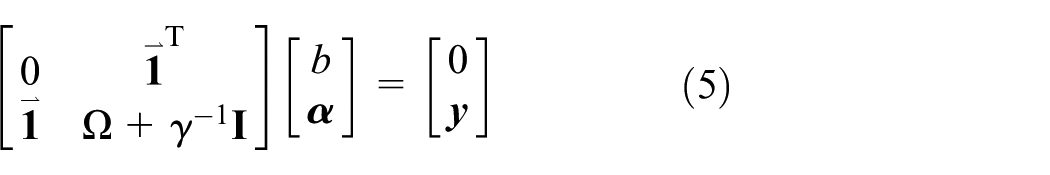
where $\overset{⇀}{1} = {[1, \dots, 1]}^{T}$ , $α = [α_{1}, \dots, α_{N}]^{T}$ , and $y = [y_{1}, \dots, y_{N}]^{T}$ . Then, Mercer’s theorem is applied within the Ω matrix

Ω_{ij} = φ {(x_{i})}^{T} φ (x_{j}) = K (x_{i}, x_{j}), i, j = 1, \dots, N

(6)

Finally, the LS-SVM regression model used for prediction can be expressed as

y (x) = \sum_{i = 1}^{N} α_{i} K (x, x_{i}) + b

(7)

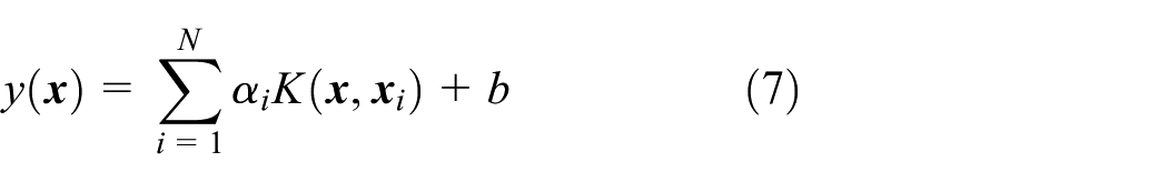
where α_i is the weight of the ith vector and K( x , x _i) represents a kernel function that transforms the nonlinear samples in the original space into linear vectors in a high-dimensional space in order to solve the linearly inseparable problem. The kernel functions commonly used include linear, polynomial, and RBF (radial basis function). In this article, we will use the RBF kernel which can result in satisfactory overall performance in cases where prior knowledge is unavailable.¹⁴

Bayesian inference theory

In practice, cross validation is often adopted to determine the model structure H (LS-SVM with kernel function K) and the regularization parameter γ of LS-SVM regression model. However, the cross-validation method needs to be performed repeatedly, which requires significant computational time. To overcome the challenge, the Bayesian framework is employed to the LS-SVM regression to obtain the kernel function parameter, regularization parameter γ, and model parameters w and e through three levels of inference. This method has been successfully applied to estimate nonlinear models for financial time series and the related volatility.²⁰

In machine learning, the RBF kernel, or Gaussian kernel, is a popular kernel function used in various kernel-based learning algorithms. The RBF kernel in a general form is

K (x_{i}, x_{j}) = \exp (\frac{- {‖ x_{i} - x_{j} ‖}^{2}}{σ^{2}})

(8)

where σ is the kernel parameter. The RBF kernel is selected in this article for the following reasons:

Large deviations will not appear when solving a linearly inseparable problem.

It possesses universality for its applicability for samples that follow any kinds of distributions as long as its parameters are reasonably determined.

In order to carry out interval prediction using the LS-SVM model, we assume that model parameter w and error vector e , respectively, obey the following Gaussian prior distribution^14,20

w ~ Norm (0, \frac{1}{μ} I_{k}), e ~ Norm (0, \frac{1}{ζ} I_{N})

(9)

where I _k and I _N are the k-by-k and N-by-N identity matrices, respectively, and 1/µ and 1/ζ are the variances of w_i (i = 1,2, …, k) and e_j (j = 1,2, …, N), respectively.

Then, the objective function (2) can be reformulated as

J (w, e) = μ E_{w} + ζ E_{D}

(10)

where µ and ζ are also called as regularization parameters, and γ = ζ/µ.²⁰Equation (10) can make the variances of w and e equal.

As a result, the LS-SVM regression model H has the following parameters that need to be inferred from the training data set S: w , b, µ, ζ, and σ. The procedure of Bayesian framework with three levels of inference can be briefly described as follows:^14,20

Level 1. Inference of model parameters w and b

Given the training data set S and regularization parameters µ and ζ of model H, the estimates, denoted by w _MP and b_MP, of model parameters w and b can be obtained by maximizing the posterior probability (11)

p (w, b | S, μ, ζ, H) = \frac{p (S | w, b, μ, ζ, H)}{p (S | μ, ζ, H)} p (w, b | μ, ζ, H)

(11)

where p(S | w , b, µ, ζ, H) is the likelihood at this level, and the evidence p(S|µ, ζ, H) is the normalizing factor. p( w , b | µ, ζ, H) is the joint prior probability distribution of w and b. In this article, w and b are assumed to be independent. A uniform distribution is used as the prior distribution for b, so p( w , b | µ, ζ, H) can be obtained considering the distribution of w given in equation (9).

Level 2. Inference of regularization parameters µ and ζ

The estimates of regularization parameters µ and ζ, denoted by µ_MP and ζ_MP, are obtained from the training data set S by applying Bayes’ rule at the second level

p (μ, ζ | S, H) = \frac{p (S | μ, ζ, H)}{p (S | H)} p (μ, ζ, H)

(12)

where a flat, non-informative prior is assumed for µ and ζ. The probability p(S | µ, ζ, H) is the same as in equation (11).

Level 3. Inference of kernel parameter σ

It is easy to see that

p (H | S) = \frac{p (S | H)}{p (S)} p (H) \propto p (S | H)

(13)

Then, the optimal value of RBF kernel parameter σ can be found by maximizing the model evidence p(S|H).

It is worth pointing out that at each level of the Bayesian framework, one has

Posterior = \frac{Likelihood}{Evidence} \times Prior

(14)

and the likelihood at a certain level equals the evidence at the previous level. In this way, by gradually integrating out the parameters at different levels, the subsequent levels are linked to each other. Interested readers can refer to Suykens and colleagues^14,20 for more details.

Interval estimate of Bayesian LS-SVM regression

After finding all the model parameters, the interval prediction of LS-SVM regression can be performed. By taking expectation on both sides of equation (1), the point estimate of LS-SVM regression model can be obtained as

y_{MP} (x) = w_{MP}^{T} φ (x) + b_{MP}

(15)

where w _MP and b_MP are the optimal model parameters obtained by Bayesian inference, and y_MP( x ) is the point estimate of y( x ) for x .

Let y_N_+ 1 be the observed value at time N + 1; then, it can be expressed as

y_{N + 1} = y_{MP} (x_{N + 1}) + e_{N + 1}

(16)

where e_N_+ 1 is the error term at time N + 1, which is assumed to follow the normal distribution with zero mean and variance 1/ζ_MP. Then, the mean and variance of y_N_+ 1 can be obtained as

E (y_{N + 1}) = y_{MP} (x_{N + 1})

(17)

Var (y_{N + 1}) = Var (y_{MP} (x_{N + 1})) + \frac{1}{ζ_{MP}}

(18)

According to Suykens et al.,¹⁴ one obtains

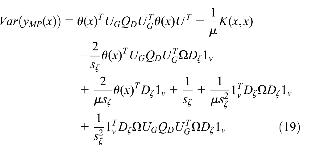
\begin{matrix} Var (y_{MP} (x)) = & θ (x)^{T} U_{G} Q_{D} U_{G}^{T} θ (x) U^{T} + \frac{1}{μ} K (x, x) \\ - \frac{2}{s_{ζ}} θ (x)^{T} U_{G} Q_{D} U_{G}^{T} Ω D_{ζ} 1_{v} \\ + \frac{2}{μ s_{ζ}} θ (x)^{T} D_{ζ} 1_{v} + \frac{1}{s_{ζ}} + \frac{1}{μ s_{ζ}^{2}} 1_{v}^{T} D_{ζ} Ω D_{ζ} 1_{v} \\ + \frac{1}{s_{ζ}^{2}} 1_{v}^{T} D_{ζ} Ω U_{G} Q_{D} U_{G}^{T} Ω D_{ζ} 1_{v} \end{matrix}

(19)

where Q_D = (µI + D_G)⁻¹ − µ⁻¹I; θ(x) = [K(x, x₁), …, K(x, x_N)]; Ω_kl = K(x_k, x_l) = ϕ(x_k)^Tϕ(x_l), where k, l = 1, 2, …, N; 1_v = [1, 1, …, 1]_v; $s_{ζ} = \sum_{i = 1}^{N} ζ_{i}$ ; and U_G and D_G are related to the eigenvalue decomposition

\begin{array}{l} (D_{ζ} - \frac{1}{s_{ζ}} D_{ζ} 1_{v} 1_{v}^{T} D_{ζ}) Ω v_{G, i} = λ_{G, i} v_{G, i}, \\ i = 1, \dots, N_{eff} \leq N - 1 \end{array}

(20)

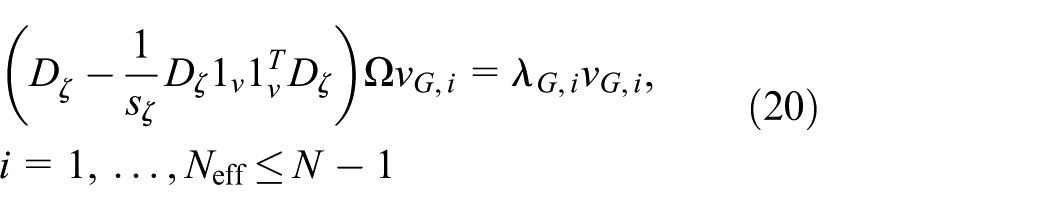
where D_G = diag([λ_{G, 1}, …, [λ_{G, Neff}]) and U_G = [(v_{G, 1}Ωv_{G, 1})^1/2v_{G, 1}, …, (v_{G, Neff}Ωv_{G, Neff})^1/2v_{G, Neff}].

Since the model parameters w and b, and the error term, all follow normal distributions, we have

P (| \frac{y_{N + 1} - E (y_{N + 1})}{\sqrt{Var (y_{N + 1})}} | \leq 1.96) = 0.95

(21)

As a result, the 95% confidence interval of y_N_+ 1 can be expressed as

[E (y_{N + 1}) - 1.96 \sqrt{Var (y_{N + 1})}, E (y_{N + 1}) + 1.96 \sqrt{Var (y_{N + 1})}]

(22)

Degradation modeling and RUL prediction using Bayesian LS-SVM

Basic architecture

Figure 1 illustrates the basic flow of using the Bayesian LS-SVM method for performance degradation modeling and lifetime prediction. First, training data and the setting algorithm parameters are used as the input to the LS-SVM framework, and then modeling begins using the LS-SVM learning algorithm on the training data. Multiple one-step predictions that constitute a degradation curve can be obtained based on this model. Meanwhile, Bayesian inference is applied to find the optimal model parameters and obtain the error bars of LS-SVM regression model. Ultimately, both point and interval estimates of RUL are obtained considering the pre-specified failure threshold.

Figure 1.

Basic architecture of RUL prediction based on Bayesian LS-SVM.

Lifetime prediction based on Bayesian LS-SVM

In the course of implementation, an iterative algorithm is introduced: training data set will be continuously updated after each one-step prediction. Specifically, each predicted value will be added into the original training set, and the updated set will be used in training to predict the value at the next point in time. The detailed procedure can be described as follows.

Let ( x _t, y_t), 1 ≤ t ≤ r, be the original training data. The values at (r + 1)th to (r + n)th time points are to be predicted. The regression equation obtained using the training data set is

y_{t} = \sum_{i = 1}^{r} α_{i} K (x_{i}, x_{t}) + b, t = 1, 2, \dots, r

(23)

Then, the one-step prediction model can be expressed as

{\hat{y}}_{r + 1} = \sum_{i = 1}^{r} α_{i} K (x_{i}, x_{r + 1}) + b

(24)

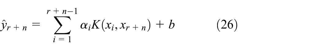
Subsequently, this predicted value can be added into the original training set. Similarly, the regression model used to predict the (r + n)th value can be expressed as

{y_{t}}^{*} = \sum_{i = 1}^{r + n - 1} α_{i} K (x_{i}, x_{t}) + b, t = 1, 2, \dots, r + n - 1

(25)

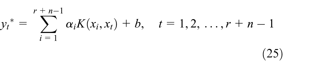
where ${y_{t}}^{*} = (y_{1}, y_{2}, \dots, y_{r}, {\hat{y}}_{r + 1}, \dots, {\hat{y}}_{r + n - 1})$ . Then

{\hat{y}}_{r + n} = \sum_{i = 1}^{r + n - 1} α_{i} K (x_{i}, x_{r + n}) + b

(26)

Implementation of RUL prediction

The RUL of an asset or system is defined as the length from the current time to the end of its useful life.⁷ The word “useful” in RUL usually implies an economic aspect which can differ significantly from the technical remaining lifetime of an asset. The technical lifetime of an industrial machine is often longer than its economic life time.²¹ Obviously, the precise definition of the useful life depends on the context and operational characteristics.

It is important to predict the RUL of a system, because it has an important role in maintenance planning, spare parts provision, operational performance, and profitability.²¹

The procedure of RUL prediction can be illustrated by Figure 2 and described as follows:

Collect training data by monitoring the asset’s performance state (often characterized by one or more key index parameters).

Train LS-SVM using the training data with a performance degradation trend being the final output; apply Bayesian inference to obtain a confidence interval while taking the uncertainties resulting from the model itself and prior information of model parameters.

Calculate both the point and interval estimates considering the given failure threshold.

Figure 2.

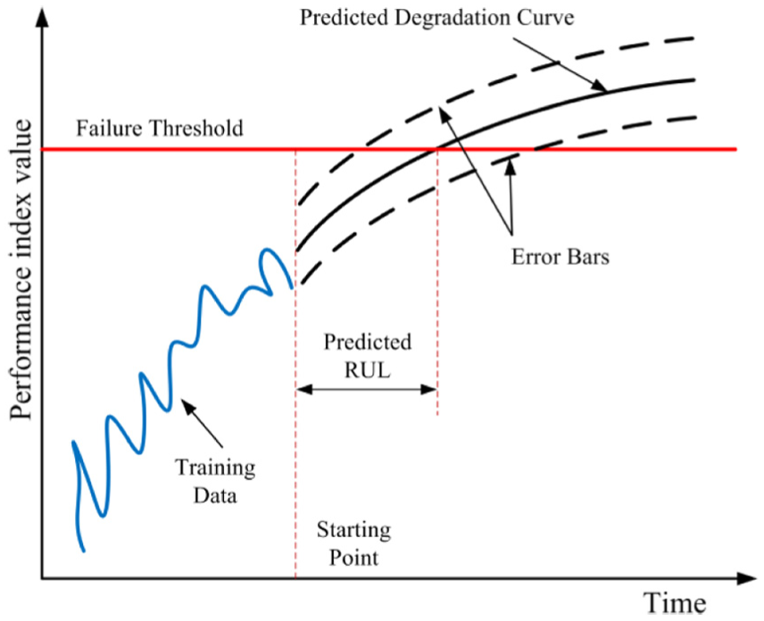
Principle of RUL prediction.

Case study and analysis

Description of data

In this section, a study on a microwave component’s degradation data is conducted to demonstrate the effectiveness of the proposed method. An important performance measure of the microwave component in this case study is the component’s power gain, which measures the ability of the component to increase the power of a signal from the input to the output. In this experiment, to model the power gain degradation of microwave component, one measurement was taken each day and a total of 361 data points were collected. From Figure 3, one can see that the degradation process exhibits a linear trend with significant fluctuation in the middle portion.

Figure 3.

Power gain’s degradation data of a microwave component.

Analysis of prediction results

In order to verify the prediction accuracy of LS-SVM, the RBF neural network (RBFNN) is used in comparison. To be more specific, the original training data set was divided into two parts. The first 200 data points were used to train LS-SVM and RBFNN, respectively, to get the predicted values of the latter 161 data points. By comparing the predicted values and real data, we can compare the prediction accuracy of these two methods.

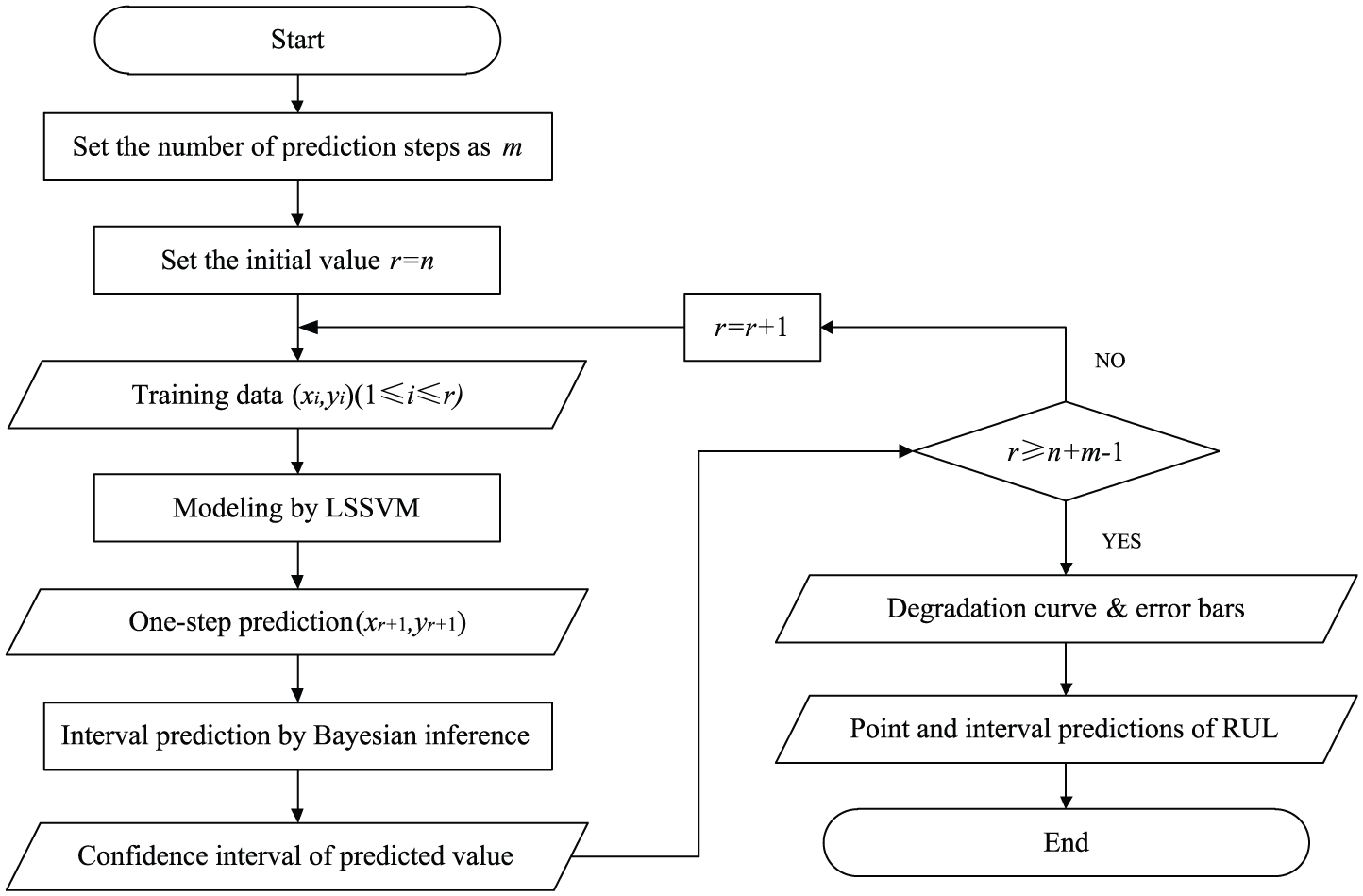
The flowchart of LS-SVM for degradation modeling is shown in Figure 4, where r (200 in this study) and n represent the number of training data points and total number of data points,²² respectively.

Figure 4.

Flowchart of Bayesian LS-SVM for degradation modeling.

Other parameters used in the procedure are as follows:

For LS-SVM, the regularization parameter is γ = 212 and the kernel function parameter is σ² = 19;

For RBFNN, the expansion rate is spread = 100 and the target of MSE is set to be goal = 0.01.

The graphical outputs of these two methods are shown in Figure 5.

Figure 5.

Graphical outputs of (a) LS-SVM and (b) RBFNN.

To make a quantitative comparison on prediction accuracy of the two methods, three accuracy indices, MAE, mean square error (MSE), and RMSE, are considered

MAE = \frac{1}{n} | e_{i} | = \frac{1}{n} \sum_{i = 1}^{n} | y_{i} - {\hat{y}}_{i} |

(27)

MSE = \frac{1}{n} \sum_{i = 1}^{n} e_{i}^{2} = \frac{1}{n} \sum_{i = 1}^{n} {(y_{i} - {\hat{y}}_{i})}^{2}

(28)

RMSE = \sqrt{\frac{1}{n} \sum_{i = 1}^{n} e_{i}^{2}} = \sqrt{\frac{1}{n} \sum_{i = 1}^{n} {(y_{i} - {\hat{y}}_{i})}^{2}}

(29)

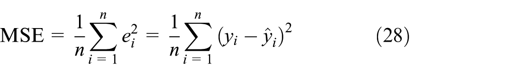
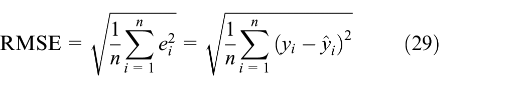
where $y_{i}$ and ${\hat{y}}_{i}$ represent the real value and the predicted value, respectively. The comparison results are listed in Table 1.

Table 1.

Comparison on precision using 200 training data.

Method	MAE	MSE	RMSE
LS-SVM	0.0661	0.0067	0.0820
RBFNN	0.1110	0.0167	0.1291

MAE: mean average error; MSE: mean square error; RMSE: root mean square error; LS-SVM: least-squares support vector machine; RBFNN: radial basis function neural network.

Then, the value of r is chosen equidistantly between 100 and 240 with the interval of 20. The corresponding results are shown in Table 2 and Figure 6.

Table 2.

Comparison on precision using different amounts of training data.

Amount of training data	LS-SVM		RBFNN
Amount of training data	MAE	MSE	MAE	MSE
100	0.0661	0.0075	0.0665	0.0076
120	0.0697	0.0082	0.0842	0.0115
140	0.0803	0.0098	0.2338	0.0720
160	0.1774	0.0377	0.7530	0.7527
180	0.2156	0.0522	0.2941	0.1453
200	0.0661	0.0067	0.1109	0.0166
220	0.0645	0.0065	0.0643	0.0064
240	0.0559	0.0049	0.0609	0.0056

LS-SVM: least-squares support vector machine; RBFNN: radial basis function neural network; MAE: mean average error; MSE: mean square error.

Figure 6.

Accuracy comparison on (a) MAE and (b) MSE.

From the results, one can see that the LS-SVM method outperforms the RBFNN method under various sizes of training data. Particularly, the RBFNN method suffers from data fluctuation (see the results when the sizes of training data are 140, 160, and 180). In contrast, the LS-SVM method is much more robust and stable.

RUL prediction using Bayesian LS-SVM

Figure 7 shows the flowchart for implementing the Bayesian LS-SVM for RUL prediction. Compared to the flowchart given in Figure 4, the main differences are as follows: (1) the original amount of training data equals the total amount of data, that is, r = n, and (2) the confidence interval is given based on Bayesian inference at each step, while the modeling principle of these two processes keeps the same.

Figure 7.

Flowchart of Bayesian LS-SVM for RUL prediction.

The parameters used in the algorithm are γ = 1000 and σ² = 500, and the failure threshold is set to be 18. The corresponding results and its partial enlarged view are shown in Figure 8. With the starting point of X = 361, the point estimate of RUL is 671 days and the 95% interval prediction is [649, 693] days.

Figure 8.

RUL prediction curve and its 95% confidence bands of microwave component: (a) RUL prediction results and (b) partial enlarged view.

Conclusion

This article provides a basic architecture for RUL prediction of a certain microwave component. The problem of LS-SVM regression under Bayesian framework with three levels of inference is analyzed, and the regression model is obtained from the past observations. Then, the point and interval estimation using the LS-SVM regression model is derived. Finally, by modeling the degradation of component’s power gain via the Bayesian LS-SVM method, both point and interval estimates of RUL are obtained. The accuracy and stability of this method are also verified by comparing the results with those of the RBF neural network.

In practice, the selection of model parameters will directly affect the accuracy of the model. Therefore, how to select the optimal model parameters is a crucial future research direction. Furthermore, selecting appropriate kernel functions for LS-SVM modeling can also be studied.

Footnotes

Academic Editor: Yongming Liu

Declaration of conflicting interests

The author(s) declared no potential conflicts of interest with respect to the research, authorship, and/or publication of this article.

Funding

The author(s) disclosed receipt of the following financial support for the research, authorship, and/or publication of this article: This work was supported in part by the National Natural Science Foundation of China (grant nos 61603018 and 61104182) and the China Scholarship Council. The work of H. Liao was supported by the US National Science Foundation under grant nos CMMI-1238301 and CMMI-1238304.

References

Lee

Zhao

. Prognostics and health management design for rotary machinery systems—reviews, methodology and applications. Mech Syst Signal Pr 2014; 42: 314–334.

Liu

Xie

Liao

. An integrated probabilistic approach to lithium-ion battery remaining useful life estimation. IEEE T Instrum Meas 2015; 64: 660–670.

Saha

Goebel

Poll

. Prognostics methods for battery health monitoring using a Bayesian framework. IEEE T Instrum Meas 2009; 58: 291–296.

Liao

Tian

A framework for predicting the remaining useful life of a single unit under time-varying operating conditions. IIE Trans 2013; 45: 964–980.

Kim

Choi

J-H.

Practical options for selecting data-driven or physics-based prognostics algorithms with reviews. Reliab Eng Syst Safe 2015; 133: 223–236.

Tsui

Chen

Zhou

. Prognostics and health management: a review on data driven approaches. Math Probl Eng 2015; 2015: 793161-1–793161-17.

Wang

. Remaining useful life estimation—a review on the statistical data driven approaches. Eur J Oper Res 2011; 213: 1–14.

Vapnik

VN.

The nature of statistical learning theory. 2nd ed.New York: Springer Science & Business Media, 2013.

Huang

Wang

. Support vector machine based estimation of remaining useful life: current research status and future trends. J Mech Sci Technol 2015; 29: 151–163.

10.

Breaz

Gao

. A modified relevance vector machine for PEM fuel-cell stack aging prediction. IEEE T Ind Appl 2016; 52: 2573–2581.

11.

Zheng

Fang

An integrated unscented Kalman filter and relevance vector regression approach for lithium-ion battery remaining useful life and short-term capacity prediction. Reliab Eng Syst Safe 2015; 144: 74–82.

12.

Liu

Zhou

Pan

. Lithium-ion battery remaining useful life estimation with an optimized Relevance Vector Machine algorithm with incremental learning. Measurement 2015; 63: 143–151.

13.

Wang

Miao

Pecht

Prognostics of lithium-ion batteries based on relevance vectors and a conditional three-parameter capacity degradation model. J Power Sources 2013; 239: 253–264.

14.

Suykens

JAK

Gestel

Brabanter

. Least squares support vector machines. Singapore: World Scientific, 2002.

15.

Khawaja

TS.

A Bayesian least squares support vector machines based framework for fault diagnosis and failure prognosis. PhD Dissertation, School of Electrical and Computer Engineering, Georgia Tech, Atlanta, GA, 2010.

16.

Wang

Zuo

Cai

. Forecasting model of engine life on wing based on LS-SVM and Bayesian inference. J Nanjing Univ Sci Technol 2013; 37: 955–959.

17.

Kamari

Hemmati-Sarapardeh

Mirabbasi

S-M

. Prediction of sour gas compressibility factor using an intelligent approach. Fuel Process Technol 2013; 116: 209–216.

18.

Ismail

Shabri

Samsudin

A hybrid model of self-organizing maps (SOM) and least square support vector machine (LSSVM) for time-series forecasting. Expert Syst Appl 2011; 38: 10574–10578.

19.

Polat

Güneş

Breast cancer diagnosis using least square support vector machine. Digit Signal Process 2007; 17: 694–701.

20.

Van Gestel

Suykens

Baestaens

. Financial time series prediction using least squares support vector machines within the evidence framework. IEEE T Neural Networ 2001; 12: 809–821.

21.

Ahmadzadeh

Lundberg

Remaining useful life estimation: review. Int J Syst Assur Eng Manag 2014; 5: 461–474.

22.

De Brabanter

Karsmakers

Ojeda

. LS-SVMlab toolbox user’s guide (version 1.8). ESAT-SISTA technical report 10-146, 2010. Leuven: KU Leuven.

A Bayesian least-squares support vector machine method for predicting the remaining useful life of a microwave component

Abstract

Keywords

Introduction

Bayesian LS-SVM theory

LS-SVM regression theory

Bayesian inference theory

Interval estimate of Bayesian LS-SVM regression

Degradation modeling and RUL prediction using Bayesian LS-SVM

Basic architecture

Lifetime prediction based on Bayesian LS-SVM

Implementation of RUL prediction

Case study and analysis

Description of data

Analysis of prediction results

RUL prediction using Bayesian LS-SVM

Conclusion

Footnotes

Declaration of conflicting interests

Funding

References