Analysis of cable effect on dynamic motion of an underwater vehicle for welding of reaction pool

Abstract

Remotely operated vehicle is a reliable tool in an emergency rescue and routing inspection of a reactor pool. In practice, a cable has been considered as an important part of a vehicle system (i.e. winch, vehicle, and cable) to evaluate and predict the mechanical characteristics, and this article presents a study on a dynamic mechanism modeling of a cable partially in water and air based on an omnidirectional motion, and a numerical simulation is employed. In this work, we programmed the model governed by a partial differential equation set, at the discrete time node which was transformed into an ordinary differential equation set regarded as an initial value problem. The dynamic mechanical characteristics of the lower endpoint (i.e. a connection point between vehicle and cable) and the upper endpoint (i.e. a connection point between cable and winch) were, respectively, quantified with acceleration and a compounded motion including a uniform and rolling motion. A dynamic-state mechanism test was carried out to verify an authenticity of the three-dimensional mechanical model and numerical solution in a circulating tank. The results demonstrated that the presented method was used to evaluate the dynamic mechanism, and held a potential to improve a vehicle design and control strategy.

Introduction

Since the Fukushima Daiichi nuclear power plant accident^1,2 in 2011, the nuclear safety has been paid attention all over the world. In a nuclear accident, the rescue focused on the nuclear reaction pool considered as a core of a power station. As unmanned equipment, an underwater vehicle has been widely used in ocean exploration, seafloor mapping, and underwater mining.^3–5 Theoretically, an underwater vehicle can be used in a daily inspection and monitoring of a reaction pool and underwater welding.

Many institutes have devoted much effort into developing an underwater vehicle for nuclear rescue. Regretfully, no vehicle has been reported until now due to some difficulties including dangerous experimental environment and a long test period. Thus, a simulation can be useful to the design and performance evaluation of an underwater vehicle. Furthermore, a cable on the tail often used to transmit signal and supply power for a vehicle was considered as a main disturbing factor. ⁶ Hence, it was critical for a simulation to analyze the mechanical characteristics of the cable.^7,8

For finding precisely the crack on walls, remotely operated vehicle (ROV) was frequently in a dynamic state. Thus, the effect of a cable force on a vehicle during motion should be considered. Recently, a plenty of works on a precise dynamic characteristic of underwater cables was presented. Generally, the mechanical model can be described by a partial differential equation (PDE) set over time and arc length of a cable, ⁹ and the numerical simulation of these flexible cables can be classified into three methods: ¹⁰ the finite difference method, the lumped mass method, and the finite element method. For example, Buckham and colleagues^11,12 presented a lumped mass model for low-tension ROV tethers, which were considered to be a system of point masses connected by visco-elastic springs, and the effects of cable’s bending and tensional stiffness were included to generate the realistic results. Zhang et al. ¹³ analyzed the characteristic of the submarine cable laying back to the seabed by a lumped mass method, which was verified by existed data. Du et al. ¹⁴ proposed a method to model the strongly nonlinear towed sonar cable array by the lumped mass method, which was simulated by fourth Runge–Kutta method applying Newton’s second law. Huo et al. ¹⁵ proposed a dynamic equation set for an underwater cable based on Euler–Bernoulli beam theory, which can be solved using finite difference method. A scale-dependent finite difference method was proposed to approximate the time fractional differential equations by Liu et al., ¹⁶ which was unconditionally stable and superior to the standard method with either uniform or non-uniform steps. Wang and Sun ¹⁷ investigated the dynamic model of a towed cable by a finite difference method, which can analyze the effect of the dynamic response of ship maneuver on the cable system maneuverability. Eidsvik and Ingrid ¹⁸ developed a novel three-dimensional cable model for ROV using Euler–Bernoulli beam theory taking account into the most important effects related to the response of underwater cables and ROVs, which was solved by the Galerkin finite element method. Quan et al. ¹⁹ presented a weak form of a cable system derived by the virtual work principle, and a formulation of the consistence linearization was spatially discredited by the finite element method. Li et al. ²⁰ presented the singular boundary method to reduce discretization errors of the PDE, which was verified the effectiveness by several benchmark examples. Fang et al. ²¹ presented a new finite element model that provided a representation of both the bending and tensional effects, and the cubic spline interpolation function was applied for the trial solution. In addition, Baleanu and colleagues^22,23 proposed an efficient numerical method based on the fractional calculus applying for a biomedical model. However, the dynamic-state mechanism of an underwater cable had figured out some achievements, but these cables mentioned in the work above were all used in sea (the open-water domain), and in this scenario, an invariable proportion between the cable length in air and in water was lower, which can result in neglecting the effect of medium fluctuation in the dynamic mechanical model. And, the cable torsion from a more angle had been not considered without the roll motion of a vehicle. Also, all results of the dynamic mechanical properties of cables were based on the simulation, which cannot ensure correctness of the model. Therefore, a dynamic-state mechanical characteristic of a cable was established based on the medium fluctuation and an omnidirectional motion of a vehicle. And then, an experiment of a cable force was conducted to verify the simulation and the model in a circulating tank.

Recently, we have developed ROV for underwater welding as shown in Figure 1. In this work, the numerical simulation was employed to quantify and predict the dynamic-state mechanical properties of the variable length cable. We set up a dynamic-state theoretical model of a cable partially in reaction pool water and air. The numerical model was described by a PDE set which can be transformed into an ordinary differential equation (ODE) set by an equal interval temporal discretization. At every time node, the ODE set—which was considered as an initial value problem—was solved in according to a state value of the lower endpoint. The dynamic-state mechanical characteristics (i.e. the tension, bi-normal shear force, normal shear force, torsion moment, bi-normal moment, normal moment, and configuration) of a cable were quantified under a constant acceleration motion and a compounded motion. Finally, a dynamic mechanism test of a cable in a circulating tank was carried out to verify the theoretical model and the numerical solution. The results demonstrated that the presented method can be used to evaluate the effect on a dynamic-state motion of ROV and held a potential to improve the design and control strategy of an underwater vehicle.

Figure 1.

A prototype of an underwater vehicle and a winch: (a) a prototype of an underwater vehicle and (b) a prototype of a winch.

The design of vehicle and cable

In previous research, many underwater vehicles have been developed. Liu et al. ²⁴ designed a new multi-functional and model-switched ROV for a decomposition of an underwater structure at sea. Miao et al. ²⁵ presented a small inspection-class underwater vehicle that carried a video camera for an underwater inspection. Anwar et al. ²⁶ designed a portable low-cost ROV that conducted survey in a shallow water.

Most recently, an open-frame underwater vehicle for welding cracked walls of a nuclear power pool in emergency and a routine inspection was designed and manufactured. The main parameters of a vehicle are shown in Table 1.

Table 1.

The main parameters of an underwater vehicle.

Symbol	Value	Remarks
L × B × H	1.06 × 0.65 × 0.66 m	The size of a vehicle
M	117 kg	The mass of a vehicle
V	0.21 m3	The volume of a vehicle

The body of an underwater vehicle included the following: a main frame, two pressure cabins, eight propellers, and buoyancy material. The cable—the diameter of which was 28 mm—can transfer signals and power for the body and welding actuators. The cable was composed of an outer sheath, armored, an inner sheath, an aluminum sheath, an insulating layer, and a cabling. The withdrawal and deployment of a cable were operated by a winch on the shore with a vehicle movement. A prototype of an underwater vehicle and a winch are shown in Figure 1.

Theoretical modeling and solution

In general, a safe distance between the water surface and a pool shore in the vertical direction (z-axis) was employed to ensure the safety of a nuclear power pool as shown in Figure 2. To describe the theoretical model precisely, the cable was divided into two parts: l₁ in water and l₂ in air. The intersection between the cable and the water surface was called as an entry water point P, and the angle between the tangle line through point P and the water surface was called as the entry angle α. A fixed coordinate system O-xyz was established, which the origin O was on the water surface. A local coordinate system b - t - n attached on the cable was established, and the tangential direction of the cable was t , the normal direction was n , and the direction b can be obtained by the right-hand rule.

Figure 2.

A fixed coordinated system and a local coordinate system.

The attitude of a cable was depicted by the Euler angles: θ, φ, and γ. The angle θ between the tangential projection and x-axis was represented as an azimuth angle, the angle φ between the tangent and xoy plane was an elevation angle, and the angle γ was a twist angle. The water depth in the reactor pool was indicated h.

The transformation from a fixed coordinate to a local coordinate was conducted under a set of rotations as Euler angles. The following rotation sequence was chosen in this section: first, rotated the local axis by the angle γ about the t -axis, then rotated the local axis by the angle φ about the b -axis, and finally rotated the local axis by the angle θ about the n -axis. A transformation matrix can be expressed as following

$$(x,y,z{)}^T=[\mathit{A}](\mathit{b},\mathit{t},\mathit{n}{)}^T$$

(1)

where the transformation matrix A between a local coordinate system and a fixed coordinate system can be indicated as

$$\mathit{A}=\left[\begin{array}{ccc}\cos \theta \cos \gamma -\sin \theta \sin \phi \sin \gamma \hfill & \sin \theta \cos \phi \hfill & -\cos \theta \sin \gamma -\sin \theta \sin \phi \cos \gamma \hfill \\ \multicolumn{1}{c}{-\sin \theta \cos \gamma -\cos \theta \sin \phi \sin \gamma }& \cos \theta \cos \phi \hfill & \sin \theta \sin \gamma -\cos \theta \sin \phi \cos \gamma \hfill \\ \multicolumn{1}{c}{\cos \phi \sin \gamma }& \sin \phi \hfill & \cos \phi \cos \gamma \hfill \end{array}\right]$$

(2)

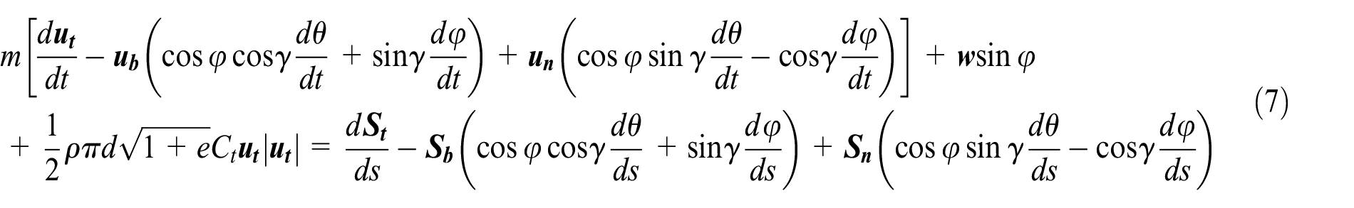
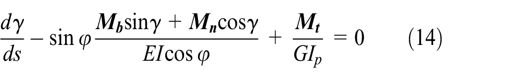
The governing equation set of the cable had been investigated by innumerable authors such as Liu et al., ²⁷ Wang and Sun, ¹⁷ and Mai et al. ²⁸ based on an invariable proportion between the cable length in air and in water. In this article, the part l₁ in water and the part l₂ were, respectively, modeled with the medium fluctuation, and the torsion was considered in this model due to an omnidirectional motion of a vehicle, which the vehicle cannot roll in past literature works. In order to simplify problems, the following assumptions were made in formulation: the cable was continuous and flexible; the section remained circular after deformation; the cable material was homogeneous, isotropic, and linearly elastic; a linear relation between tension and strain was kept; and the cable was always in tension. Taking part l₁ as an example, the dynamic-state equations of a cable element can be represented as in a local coordinate system

$$\frac{d{\mathit{M}}_{\mathit{b}}}{\mathrm{ds}}+{\mathit{M}}_{\mathit{n}}\frac{{\mathit{M}}_{\mathit{t}}}{G{I}_p}-{\mathit{M}}_{\mathit{t}}\frac{{\mathit{M}}_{\mathit{n}}}{\mathrm{EI}}+{\mathit{S}}_{\mathit{n}}{(1+\frac{{\mathit{S}}_{\mathit{t}}}{\mathrm{EA}})}^3=0$$

(3)

$$\frac{d{\mathit{M}}_{\mathit{t}}}{\mathrm{ds}}=0$$

(4)

$$\frac{d{\mathit{M}}_{\mathit{n}}}{\mathrm{ds}}+{\mathit{M}}_{\mathit{t}}\frac{{\mathit{M}}_{\mathit{b}}}{\mathrm{EI}}-{\mathit{M}}_{\mathit{b}}\frac{{\mathit{M}}_{\mathit{t}}}{G{I}_p}-{\mathit{S}}_{\mathit{b}}{(1+\frac{{\mathit{S}}_{\mathit{t}}}{\mathrm{EA}})}^3=0$$

(5)

$$\begin{array}{c}m[\frac{d{\mathit{u}}_{\mathit{b}}}{\mathrm{dt}}-{\mathit{u}}_{\mathit{n}}(\sin \phi \frac{d\theta }{\mathrm{dt}}+\frac{d\gamma }{\mathrm{dt}})+{\mathit{u}}_{\mathit{t}}(\cos \phi \cos \gamma \frac{d\theta }{\mathrm{dt}}+\sin \gamma \frac{d\phi }{\mathrm{dt}})]+\mathit{w}\cos \phi \sin \gamma \hfill \\ +\frac{1}{2}\rho d\sqrt{1+e}{C}_b{\mathit{u}}_{\mathit{b}}\sqrt{{\mathit{u}}_{\mathit{b}}^2+{\mathit{u}}_{\mathit{n}}^2}=\frac{d{\mathit{S}}_{\mathit{b}}}{\mathrm{ds}}+{\mathit{S}}_{\mathit{t}}(\cos \phi \cos \gamma \frac{d\theta }{\mathrm{ds}}+\sin \gamma \frac{d\phi }{\mathrm{ds}})-{\mathit{S}}_{\mathit{n}}(\sin \phi \frac{d\theta }{\mathrm{ds}}+\frac{d\gamma }{\mathrm{ds}})\hfill \end{array}$$

(6)

$$\begin{array}{c}m[\frac{d{\mathit{u}}_{\mathit{t}}}{\mathrm{dt}}-{\mathit{u}}_{\mathit{b}}(\cos \phi \cos \gamma \frac{d\theta }{\mathrm{dt}}+\sin \gamma \frac{d\phi }{\mathrm{dt}})+{\mathit{u}}_{\mathit{n}}(\cos \phi \sin \gamma \frac{d\theta }{\mathrm{dt}}-\cos \gamma \frac{d\phi }{\mathrm{dt}})]+\mathit{w}\sin \phi \hfill \\ +\frac{1}{2}\rho \pi d\sqrt{1+e}{C}_t{\mathit{u}}_{\mathit{t}}\left|{\mathit{u}}_{\mathit{t}}\right|=\frac{d{\mathit{S}}_{\mathit{t}}}{\mathrm{ds}}-{\mathit{S}}_{\mathit{b}}(\cos \phi \cos \gamma \frac{d\theta }{\mathrm{ds}}+\sin \gamma \frac{d\phi }{\mathrm{ds}})+{\mathit{S}}_{\mathit{n}}(\cos \phi \sin \gamma \frac{d\theta }{\mathrm{ds}}-\cos \gamma \frac{d\phi }{\mathrm{ds}})\hfill \end{array}$$

(7)

$$\begin{array}{c}m[\frac{d{\mathit{u}}_{\mathit{n}}}{\mathrm{dt}}+{\mathit{u}}_{\mathit{b}}(\sin \phi \frac{d\theta }{\mathrm{dt}}+\frac{d\gamma }{\mathrm{dt}})+{\mathit{u}}_{\mathit{t}}(-\cos \phi \sin \gamma \frac{d\theta }{\mathrm{dt}}+\cos \gamma \frac{d\phi }{\mathrm{dt}})]+\mathit{w}\cos \phi \cos \gamma \hfill \\ +\frac{1}{2}\rho d\sqrt{1+e}{C}_n{\mathit{u}}_{\mathit{n}}\sqrt{{\mathit{u}}_{\mathit{n}}^2+{\mathit{u}}_{\mathit{b}}^2}=\frac{d{\mathit{S}}_{\mathit{n}}}{\mathrm{ds}}+{\mathit{S}}_{\mathit{b}}(\sin \phi \frac{d\theta }{\mathrm{ds}}+\frac{d\gamma }{\mathrm{ds}})+{\mathit{S}}_{\mathit{t}}(-\cos \phi \sin \gamma \frac{d\theta }{\mathrm{ds}}+\cos \gamma \frac{d\phi }{\mathrm{ds}})\hfill \end{array}$$

(8)

$$\begin{array}{c}(1+e)(\cos \phi \cos \gamma \frac{d\theta }{\mathrm{dt}}+\sin \gamma \frac{d\phi }{\mathrm{dt}})-(1+e)\frac{{\mathit{M}}_{\mathit{n}}}{\mathrm{EI}}=\frac{d{\mathit{u}}_{\mathit{b}}}{\mathrm{ds}}-{\mathit{u}}_{\mathit{n}}(\sin \phi \frac{d\theta }{\mathrm{ds}}+\frac{d\gamma }{\mathrm{ds}})\hfill \\ +{\mathit{u}}_{\mathit{t}}(\cos \phi \cos \gamma \frac{d\theta }{\mathrm{ds}}+\sin \gamma \frac{d\phi }{\mathrm{ds}})\hfill \end{array}$$

(9)

$$\begin{array}{cc}\multicolumn{1}{c}{\frac{1}{\mathrm{EA}}\frac{d{\mathit{S}}_{\mathit{t}}}{\mathrm{dt}}=}& \frac{d{\mathit{u}}_{\mathit{t}}}{\mathrm{ds}}-{\mathit{u}}_{\mathit{b}}(\cos \phi \cos \gamma \frac{d\theta }{\mathrm{ds}}+\sin \gamma \frac{d\phi }{\mathrm{ds}})\hfill \\ \multicolumn{1}{c}{}& +{\mathit{u}}_{\mathit{n}}(\cos \phi \sin \gamma \frac{d\theta }{\mathrm{ds}}-\cos \gamma \frac{d\phi }{\mathrm{ds}})\hfill \end{array}$$

(10)

$$\begin{array}{c}(1+e)(-\cos \phi \sin \gamma \frac{d\theta }{\mathrm{dt}}+\cos \gamma \frac{d\phi }{\mathrm{ds}})+(1+e)\frac{{\mathit{M}}_{\mathit{n}}}{\mathrm{EI}}=\frac{d{\mathit{u}}_{\mathit{n}}}{\mathrm{ds}}\hfill \\ +{\mathit{u}}_{\mathit{t}}(-\cos \phi \sin \gamma \frac{d\theta }{\mathrm{ds}}+\cos \gamma \frac{d\phi }{\mathrm{ds}})+{\mathit{u}}_{\mathit{b}}(\sin \phi \frac{d\theta }{\mathrm{ds}}+\frac{d\gamma }{\mathrm{ds}})\hfill \end{array}$$

(11)

$$\frac{d\theta }{\mathrm{ds}}+\frac{{\mathit{M}}_{\mathit{b}}\sin \gamma +{\mathit{M}}_{\mathit{n}}\cos \gamma }{\mathrm{EI}\cos \phi }=0$$

(12)

$$\frac{d\phi }{\mathrm{ds}}-\frac{{\mathit{M}}_{\mathit{b}}\cos \gamma -{\mathit{M}}_{\mathit{n}}\sin \gamma }{\mathrm{EI}}=0$$

(13)

$$\frac{d\gamma }{\mathrm{ds}}-\sin \phi \frac{{\mathit{M}}_{\mathit{b}}\sin \gamma +{\mathit{M}}_{\mathit{n}}\cos \gamma }{\mathrm{EI}\cos \phi }+\frac{{\mathit{M}}_{\mathit{t}}}{G{I}_p}=0$$

(14)

In equations above, the unknowns to be solved were S_b , S_t , S_n , M_b , M_t , M_n , u_b , u_t , u_n , θ, φ, and γ. S_b and S_n were, respectively, shear force in the bi-normal direction and the normal moment; S_t is the tension; M_b and M_n , respectively, were the bi-normal moment and normal moment; M_t is the torsional moment. u_b , u_t , and u_n were, respectively, the bi-normal, tangential, and normal velocity of the cable. C_b, C_t, and C_n were, respectively, the bi-normal, tangential, and normal hydrodynamic coefficients. m is the mass of a cable per unit length. w is the cable weight per unit in water. E is an elasticity modulus, I is the moment of inertia of a cross section, A is the cross-sectional area of the cable, G is the shear modulus, I_p is the polar moment of inertia of a cross section, and d is the cable diameter. e is the cable strain and e =  S_t /(EA).

According to equations (3)–(14), a matrix format of a PDE set can be written as

$${\mathit{M}}_{12\times 12}\frac{\partial {\mathit{Y}}_{12\times 1}}{\partial s}={\mathit{N}}_{12\times 12}\frac{\partial {\mathit{Y}}_{12\times 1}}{\partial t}+{\mathit{Q}}_{12\times 1}$$

(15)

where

$$Y={(S_b,S_t,S_n,M_b,M_t,M_n,u_b,u_t,u_n,\theta ,\phi ,\gamma )}^T$$

(16)

The coefficient matrix of the unknowns to arc length differential and time differential were, respectively, M and N . The term irrelevant to the unknowns to arc or time differential was Q .

In generally, the PDE set (15) was discretized by a finite difference method in time. Assume that the time was divided into a series of time steps Δt which was infinitesimal. At every time node, the cable was deemed to be in a quasi-steady state due to a sufficiently small time step. Equations (9)–(11) were from the consistent equation were replaced by

$$\frac{\mathrm{dx}}{\mathrm{ds}}=(1+e)\cos \phi \cos \theta$$

(17)

$$\frac{\mathrm{dy}}{\mathrm{ds}}=(1+e)\cos \phi \sin \theta$$

(18)

$$\frac{\mathrm{dz}}{\mathrm{ds}}=(1+e)\sin \phi$$

(19)

Hence, the PDE set was transformed into a series of ODEs, which was written as

$$\{\begin{array}{c}t=0:{\mathit{K}}_{0j}\frac{\partial {\mathit{Y}}_{0j}}{\partial s}+{\mathit{Q}}_{0j}=0\hfill \\ \multicolumn{1}{c}{t=1:{\mathit{K}}_{1j}\frac{\partial {\mathit{Y}}_{1j}}{\partial s}+{\mathit{Q}}_{1j}=0}\\ \multicolumn{1}{c}{⋮}\\ \multicolumn{1}{c}{t=i-1:{\mathit{K}}_{(i-1)j}\frac{\partial {\mathit{Y}}_{(i-1)j}}{\partial s}+{\mathit{Q}}_{(i-1)j}=0}\\ \multicolumn{1}{c}{t=i:{\mathit{K}}_{\mathrm{ij}}\frac{\partial {\mathit{Y}}_{\mathrm{ij}}}{\partial s}+{\mathit{Q}}_{\mathrm{ij}}=0}\end{array}$$

(20)

where superscript i marked ith time step. The cable in space was divided into n segments of length Δs, thus the variables at the jth node were Y _j  = [S_bj, S_tj, S_nj, M_bj, M_tj, M_nj, x_j, y_j, z_j, θ_j, φ_j, γ_j] ^T , j ∈ [0, n]. K_ij was the coefficients matrix of the unknowns to arc differential under a quasi-steady state. Therefore, a series of ODE sets which were from equation (15) can be obtained. The numerical solution of an ODE set cannot be obtained by itself. An initial condition which was a state value of an endpoint or any point of a cable was added to solve ODE sets. For the part l₁, the state value of a lower endpoint can be obtained according to a vehicle motion. On the basis of the transformation between a fixed coordinate system and a local coordinate system, the initial force value of the low endpoint was

$$\begin{array}{cc}\multicolumn{1}{c}{{\mathit{S}}_{\mathit{b}0}=}& (\cos \theta \cos \gamma -\sin \theta \sin \phi \sin \gamma ){\mathit{F}}_{\mathit{x}}\hfill \\ \multicolumn{1}{c}{}& -(\sin \theta \cos \gamma +\cos \theta \sin \phi \sin \gamma ){\mathit{F}}_{\mathit{y}}+\cos \phi \sin \gamma {\mathit{F}}_{\mathit{z}}\hfill \end{array}$$

(21)

$${\mathit{S}}_{\mathit{t}0}=\sin \theta \cos \phi {\mathit{F}}_{\mathit{x}}+\cos \theta \cos \phi {\mathit{F}}_{\mathit{y}}+\sin \phi {\mathit{F}}_{\mathit{z}}$$

(22)

$$\begin{array}{cc}\multicolumn{1}{c}{{\mathit{S}}_{\mathit{n}0}}& =(-\cos \theta \sin \gamma -\sin \theta \sin \phi \cos \gamma ){\mathit{F}}_{\mathit{x}}\hfill \\ \multicolumn{1}{c}{}& +(\sin \theta \sin \gamma -\cos \theta \sin \phi \cos \gamma ){\mathit{F}}_{\mathit{y}}+\cos \phi \cos \gamma {\mathit{F}}_{\mathit{z}}\hfill \end{array}$$

(23)

where F_x , F_y , and F_z were external forces on a vehicle obtained by computational fluid dynamics (CFD).^29–31 A cable was connected to the vehicle through a hinge; hence, the initial value M_b0, and M_n0 can be set as 0, and the initial value of the torsion moment M_t0 was equal to the resistance moment under a roll motion, which can be obtained by CFD. The initial value of azimuth angle θ₀ was the angle between the motion direction of a vehicle and the y-axis, an initial value of the elevation angle φ₀ was equal to the entry water angle α.

The dynamic mechanical model of part l₂ is nearly the same as that of part l₁, and the unique difference is the density. A part l₂ was connected with a part l₁ by the entry water point P, that is, the point P was the upper endpoint of l₁, and was lower endpoint of l₂ synchronously. The state value of point P can be obtained by calculation and then the state value was considered as the initial value of a government equation set of the part l₂.

However, unlike a typical towed cable system, where the cable length was fixed, the length was not fixed as it was gradually deployed or withdrawal by a winch. Hence, the length change of the part l₁ and l₂ can result in the variation of an integral region of equation (15), and the number of segments of l₁ and l₂ was altered during deployment or withdrawal as depicted in Figure 3.

Figure 3.

The length change of cable during deployment or withdrawal.

The relationship between the distance from a vehicle to a winch in the y-axis and time with a motion can be written as

$$L(t_i)=s_0+\sum _{i}s(t_i)$$

(24)

where s₀ was the initial distance between a vehicle and a winch in the y-axis, s(t_i) was a motion distance, L(t_i) was the distance between a vehicle and a winch in the y-axis at the time step t_i. According to the geometry relation shown in Figure 3, we can obtain

$$\alpha (t_i)=\arctan \frac{h_0+h_1}{L(t_i)}$$

(25)

where h₁ was a height between a winch and the water surface, h₀ was a height between a vehicle and the water surface, and α(t_i) was the entry water angle at the time step t_i. Hence, the formula of a cable length in water or air with time t can be obtained

$$l_{i2}=\frac{h_1}{\sin [\alpha (t_i)]}$$

(26)

$$l_{i1}=\frac{h_1+h_0}{\sin [\alpha (t_i)]}-l_{i2}$$

(27)

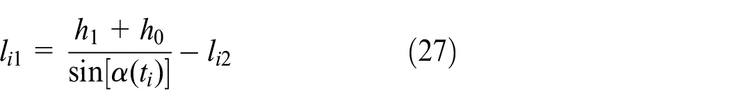
where l_i1 was the length in water and l_i2 was the length in air at the time step t_i.

Simulation and discussion

To seek for the cracks accurately most of time, an underwater vehicle was in the dynamic state. We picked the bi-normal force S_b , the tension S_t , the normal force S_n , the bi-normal moment M_b , the torsion M_t , the normal moment M_n , and the configuration to investigate the dynamic-state mechanical characteristics, which was directly related to the velocity.

An underwater vehicle (Figure 1) moved along the y-axis in line, hence the initial value of azimuth angle θ₀ was set to be 0° consistently. The position of a winch on the shore was set as (x, y, z) _N  = (0, 0, 0). The physical characteristics of the cable were as follows: the diameter d = 0.028 m, the mass per length m = 0.95 kg/m, the bi-normal coefficient C_b = 1.44; the tangential coefficient C_t = 0.15, the normal coefficient C_n = 1.44, the elasticity modulus E = 550 GPa, the shear modulus G = 180 GPa, and Poisson’s ratio P_v = 0.5.

Acceleration motion

It was assumed that an underwater vehicle accelerated under 0.01 m/s² from 0 m/s to the final velocity 0.4 m/s can result in the cable deployment. The time t was discretized by an equal step. The resistance at every time node can be calculated by CFD. And other condition was that the water depth was 20 m, the entry water degree was 30°, and the cable initial length was 30 m. By calculating the tension S_t , the normal shear force S_n , the bi-normal moment M_b , and the configuration can be obtained, and the results are shown as Figure 4.

Figure 4.

The dynamic-state mechanical characteristics of a cable under a constant acceleration: (a) tension S_t , (b) normal force S_n , (c) bi-normal moment M_b , and (d) cable configuration in plane yoz.

The tension S_t shown in Figure 4(a) increased obviously at the upper endpoint and the lower endpoint with a constant acceleration, and there was an approximate linear relationship between tension and time. From Figure 4(b), we can find that there was a decreasing curve relationship between time and normal shear force S_b at the upper endpoint and the lower endpoint. In Figure 4(c), it was found that an obvious decrease trend on the bi-normal moment M_b was detectable at the upper endpoint, and a tiny decrease in M_b at the lower endpoint was spotted. From Figure 4(d), we can find that with a constant acceleration, there was no detectable change on the position of the lower endpoint in the z-axis.

Compounded motion

To weld and inspect side walls of a nuclear reaction pool, a vehicle can roll 90°, which made torsion on the cable. It was assumed that a vehicle moved in line along the y-axis at a velocity of 0.2 m/s with a roll of an angular velocity of 6°/s. The water depth of a reaction pool was 20 m, and the density was 1006 kg/m³. The dynamic-state mechanical characteristics of a cable (i.e. the tension, the bi-normal shear force, the normal shear force, the bi-normal moment, the torsion, and the normal moment) are depicted in Figure 5.

Figure 5.

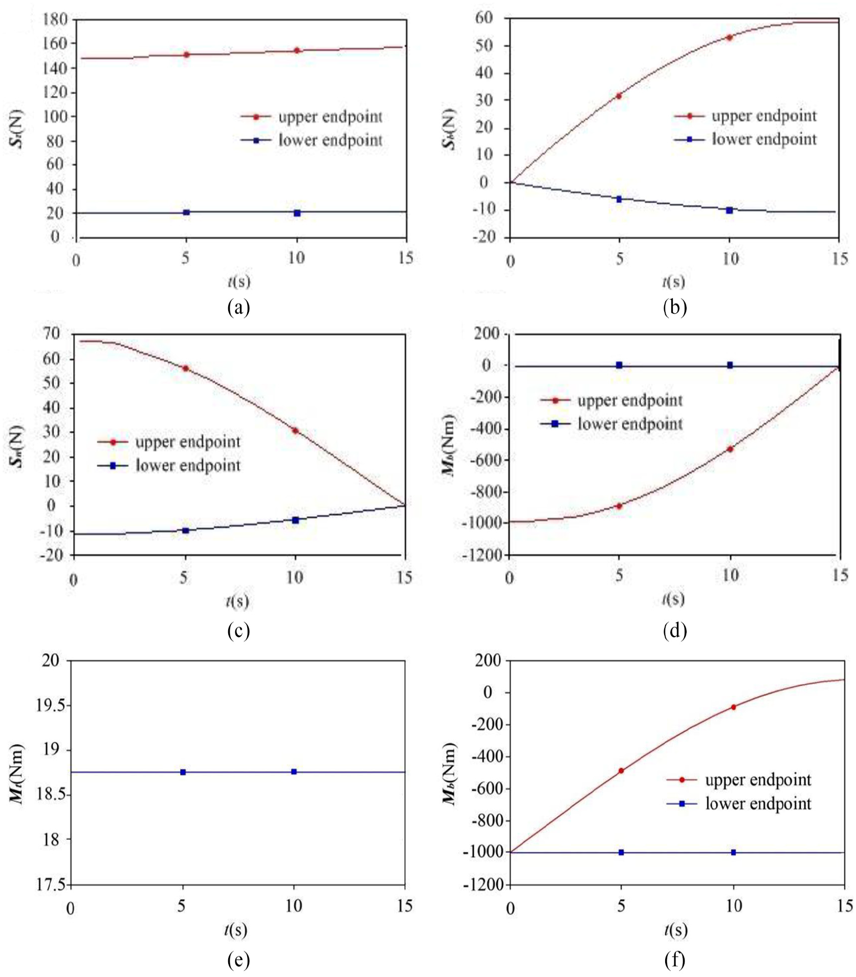
The dynamic-state mechanical characteristics of the cable under a motion compounded of a uniform motion and a rolling motion. (a) The tension S_t of the upper endpoint and the lower endpoint. (b) The bi-normal shear force S_b of the upper endpoint and the lower endpoint. (c) The normal shear force S_n of the upper endpoint and the lower endpoint. (d) The bi-normal moment M_b of the upper endpoint and the lower endpoint. (e) The torsion M_t of the upper endpoint and the lower endpoint. (f) The normal moment M_n of the upper endpoint and the lower endpoint.

In Figure 5(a), there was little change on the tension S_t at the upper endpoint and the lower endpoint with a compounded motion. From Figure 5(b), we can find that the bi-normal shear force S_b at the lower endpoint decreased with a compounded motion, but S_b at the upper endpoint shown an obvious parabolic increment with time t. From Figure 5(c), it was find that the normal shear force S_n at the lower endpoint slightly increased, while a decrease between S_n at the upper endpoint and time t was detectable. In Figure 5(d), the bi-normal moment M_b at the lower endpoint always stayed at 0 and M_b at the upper endpoint was markedly reduced. From Figure 5(e), we can find that the torsion M_t at every point of a cable was unchanged with time t. In Figure 5(f), it was found that the normal moment M_n was invariant, which was always equal to the initial value, but M_n at the upper endpoint showed a clear growth on time t.

A test of dynamic mechanism of a cable

A full-scale dynamic mechanism test of a cable carried out in a circulating tank was almost impossible due to dozens of meters long. At present, a mechanics experiment of the underwater cable was very limited, most of which was a measurement of cable resistance. In this section, the dynamic mechanical properties of the cable arranged on the vehicle were measured by a self-made cable model and a dynamic signal analyzer in a circulating tank, which can prove the correctness of a theoretical mechanical model and the validity of the numerical solution.

The test design of a cable mechanism

The test platform of a cable mechanism consisted of a data acquisition system which can monitor real-time change of a cable mechanism and the current velocity of a circulating tank. One end of a self-made cable model was arranged on the fixed frame, and the other end was always in free suspension in a circulating tank. The test platform is shown in Figure 6.

Figure 6.

A test platform of a cable force: (a) data acquisition system and (b) underwater experiment model.

In this test, a self-made cable model consisted of a physical model, a strain sensor, and an elastic base. Here, a section of the cable on the vehicle which was 2.5 m long was treated as a physical model. Four sets of strain gauge sensors were distributed equally on the section. The distances from the free end of a cable were, respectively, 0.3 m (observation point No. 1), 0.85 m (observation point No. 2), 1.4 m (observation point No. 3), and 1.95 m (observation point No. 4). At every observation point, four strain gauge sensors were uniformly arranged in the circumference. The chip and the lead connection of a sensor were uniformly sprayed insulating paint, which had an effect of sealing and waterproofing. The physical model of the cable and the arrangement of a strain gauge sensor are shown in Figure 7.

Figure 7.

The physical model of a cable: (a) arrangement schematic diagram of a self-made experimental model and (b) arrangement diagram of a strain gauge sensor.

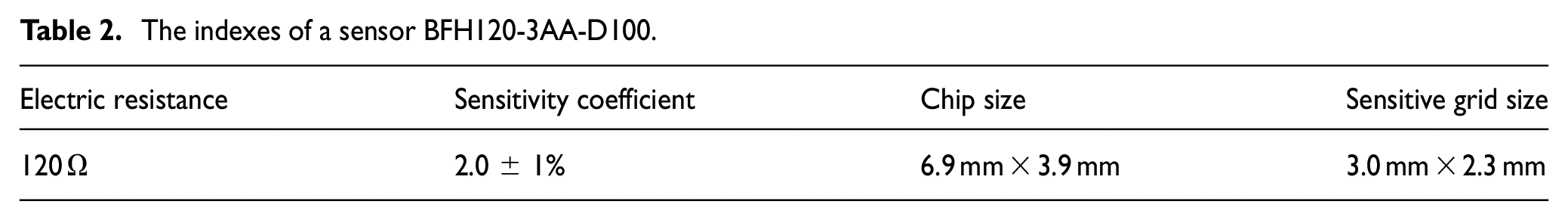
According to the vehicle operation, the flow velocity in a circulating tank was set as 0.3–0.5 m/s, which can prevent a cable rising to the water surface due to the excessive velocity and the deformation of a sensor suppressed due to the small velocity. The tension of each point of a cable was 0–15 N under the flow velocity 0.3–0.5 m/s based on the previous research,^27,32,33 which required a sensor selected with a suitable range, a high measuring accuracy, and a small size of sensitive grating. Based on all requirements above the specification of a strain gauge sensor selected were BFH120-3AA-D100, and the technical indexes are shown in Table 2.

Table 2.

The indexes of a sensor BFH120-3AA-D100.

Electric resistance	Sensitivity coefficient	Chip size	Sensitive grid size
120 Ω	2.0 ± 1%	6.9 mm × 3.9 mm	3.0 mm × 2.3 mm

The elastic base was an important component of a strain sensor, and the selection of material type followed the principles: the base produced a large deformation under a small force with a good linearity; the base was easily processed to make the shape required by a test; the base was hard to react chemically with the cable skin with a good adhesion. Through repeated experiments, the phenolic resin was selected as the elastic base material.

To obtain the relationship between the mass and a strain, the sensor was statically calibrated, that is, the strain was obtained by a dynamic signal analyzer due to the gravity from a weight loaded on the sensor. And then, the function between the mass and a strain was obtained by repeated tests. The test platform of a strain gauge sensor calibration is shown in Figure 8.

Figure 8.

A test platform of a strain gauge sensor calibration.

The weights which were, respectively, 100, 200, 300, 400, 500, 700, 1000, and 1500 g were loaded at the end of a cable to calibrate a strain gauge sensor. The strain values can be obtained as shown in Table 3.

Table 3.

The strain values of sensors under different masses.

Mass (g)	100	200	300	400	500	700	1000	1500
Strain (μm)	128.51	200.04	243.89	259.09	284.46	313.03	329.18	340.79

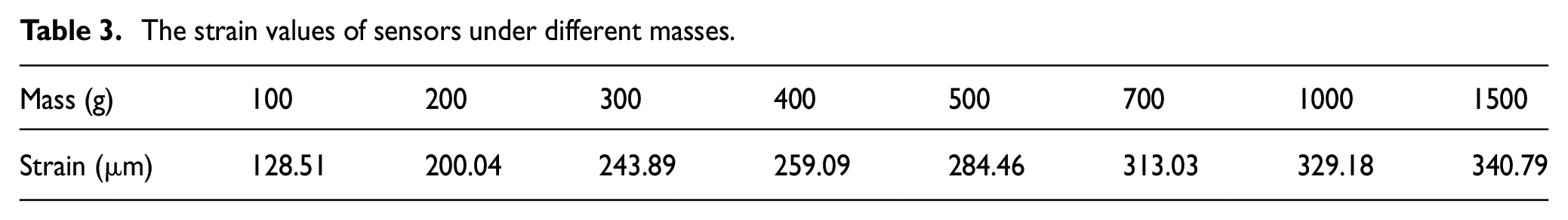
The relation between a strain and the mass can be gained by a data fitting

$$m_F=3.931\times {10}^{-12}{e}^{0.09582\mu }+23.33e^{0.01073\mu }$$

(28)

where m_F is the mass of a weight and μ is the strain.

The process and results of a test

In this section, the flow in the circulating tank accelerated from stationary to a uniform motion. In this process, the fluctuation of the cable mechanism was recorded by a dynamic signal analyzer, that is, the dynamic mechanism of a cable was obtained at any time. For the flow velocity of 0.35 m/s, the mechanical results of every observation point, respectively, obtained by the test, using the simulation in this article, in Du et al., ¹⁴ and Wang and Sun, ¹⁷ are shown in Figure 9.

Figure 9.

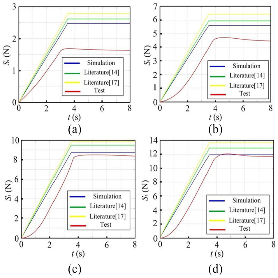
The dynamic-state mechanism of a cable at each observation point: (a) the mechanism of observation point 1, (b) the mechanism of observation point 2, (c) the dynamic mechanism of observation point 3, and (d) the dynamic mechanism of observation point 4.

From Figure 9, we can find that, during acceleration, the cable tension at each observation point shows a parabolic growth with time t. And during a uniform motion, a fluctuation of the tension at each observation point was not detectable, which was basically a line. At observation point No. 1, the error was 20% by comparing with the simulation owing to an obvious disturbance from the free end of the cable, but the more the distance from the free end was, the less the effect was. Hence, the test errors at observation point No. 2, observation point No. 3, and observation No. 4 were, respectively, 10%, 3.5%, and 1.5%. In summary, all errors were acceptable, which verified the mechanical model of a cable and the numerical simulation. In addition, the dynamic mechanical of the cable is, respectively, simulated by the methods mentioned in Du et al. ¹⁴ and Wang and Sun, ¹⁷ but the errors was more, which proved that the results in this article are significantly better than those presented in the literature.

Conclusion

In this work, the dynamic-state mechanical characteristics of the cable on the vehicle were studied. A theoretical model considering medium change was regarded as a PDE set, which can be transformed into an ODE set by an equal interval time discretization. At every time node, the ODE set which was considered as an initial value problem was solved. And then, the dynamic-state mechanical properties of the cable were quantified under a constant acceleration and a compounded motion including a uniform motion and a rolling motion. With acceleration from 0 to 0.4 m/s, the tension at the upper endpoint and the lower endpoint, respectively, climbed at 55 and 45 N, while a decrease in normal shear force was 45 and 15 N. Also, the bi-normal moment was decreased by 115 N m at the upper endpoint, and the position of the lower endpoint was increased by 1 m in the z-axis. With a compounded motion from 0 to 15 s, the tension at the lower endpoint and upper endpoint was unchanged, S_b and S_n at the lower endpoint, respectively, decreased by 10 N and increased by 20 N, and at the upper endpoint, S_b and S_n , respectively, increased by 60 N and decreased by 60 N. M_b and M_n at the lower endpoint remained 0 and at the upper endpoint increased by 60 N m, and there was no change on M_t , which was 18.75 N m with time t and arc length s. By comparing the simulation with experimental results, the authenticity of the mechanical model of a cable was verified, and the numerical solution was shown to be accurate. The results demonstrated that the presented method can be used to evaluate the dynamic-state mechanical characteristics and held a potential to improve an underwater vehicle design and control strategy. To further obtain a more reasonable mathematical model, the fractional calculus derivative can be applied, which can help us to make more realistic judgments about the complex dynamics of the real-world phenomena.