Sage Journals: Discover world-class research

Abstract

Remotely operated vehicle is a reliable and efficient tool in routing inspection of reactor pools of nuclear power plants. While, there is still no study on steady-state motion of remotely operated vehicle which is crucial for reaction pool underwater welding reported. In practice, the cable force has been considered as a critical factor affecting the vehicle’s operation. To evaluate and predict the disturbing effect caused by the cable mounted on the tailing of a vehicle, a numerical simulation can be employed. In this work, we set up a theoretical model of a cable partially in reaction pool water and air to validate the remotely operated vehicle design and reduce the prototype developing time. We programmed the model governed by an ordinary differential equation set, which was considered as an initial value problem following a dimensionless treatment to be solved. The influence by factors (i.e. velocity, water depth, entry water angle, water density and cable length on tension, normal shear force, and binormal moment) was quantified by a numerical method. The test of a cable force was carried out to verify an authenticity of the three-dimensional mechanical model and a numerical method. The results demonstrated that the presented method could be used to evaluate the effect of real environment factors on a remotely operated vehicle steady-state motion and held a potential to improve the remotely operated vehicle design and control strategy.

Keywords

Remotely operated vehicle reaction pool cable force effect environmental factors cable force test

Introduction

Since the Fukushima nuclear accident occurred in 2011, the nuclear safety has become globally a critical issue.^1,2 As an unmanned method, remotely operated vehicle (ROV) had been widely used in ocean exploration,³ seafloor mapping,⁴ deep-sea mining,⁵ and so on. In particular, ROV can be used in daily underwater inspection and monitoring of a reaction pool. Therefore, many institutes had devoted much effort into developing nuclear rescue robots.^6
–8 However, there was still no robot for a nuclear reaction pool welding reported due to dangerous experimental environment and a long-time cost. Of these, a numerical simulation can be useful to improve the mechanism design and performance for reducing time in developing ROV.

In parallel, during a whole run of reaction pool welding via ROV, a cable on the tail of the vehicle is often used to transmit signals between a remote operation panel and the vehicle and to transmit power for moving and welding. Cable force was considered as a main disturbing factor of ROV.⁹ Due to the high current power supply, the ratio of length to diameter of the cable was larger than these cable’s on other underwater vehicles,^10,11 and the disturbing effects on the body increased consequently. Earlier, there were a growing number of research on the mechanics of underwater cables for establishing precise theoretical models. Walton and Polachech¹² established a dynamic equation of suspended chain by the lumped mass method. Ablow and Schechter¹³ solved a dynamic equation of an underwater cable by a finite difference method. Millinazzo et al.¹⁴ presented an improved algorithm to enhance a computational efficiency based on Ablow’s literature, and an authenticity of the algorithm was verified by an experiment. Chiou¹⁵ proposed a direct algorithm, which a governing equation of a cable element in the local coordinate system was transformed into a two-point boundary value problem solved by the Newton–Raphson iterative method. However, all these studies were focused on the dynamic motion of a cable as the steady-state working condition was unnecessary.

For welding precisely, ROV should frequently be in a steady-state working (moving and welding). Thus, the cable force induced issues during a welding operation should be considered. De Zoysa¹⁶ established a three-dimensional equilibrium equation of an underwater towed cables. Friswell¹⁷ solved a steady-state equation in De Zoysa’s literature by the shooting method. Leech and Tabarrok¹⁸ presented a theoretical model of an underwater cable to study space shape and tension distribution in a two-dimensional steady state by an analytic method. Wang and colleagues^19,20 converted the steady-state dynamic equation into a two-point boundary value problem which was solved by a bisection method. Wang et al.^21,22 proposed a time-delay estimation element applied to properly compensate the lumped unknown dynamics due to the cable of a cable-driven manipulators system. Although these reports had figured out some mechanism issues of a cable during the steady-state operation of ROV, all results were based on the simulation, which can’t ensure accuracy. These vehicles were all used in sea (an open-water domain); in this scenario, the proportion between the cable length in water and that in air is lower, and the ratio of cable length to diameter is smaller. Also, the environment parameters (e.g. the seawater density and seawater temperature) are almost consistent at the same depth. The effect of medium fluctuation on the steady mechanical model has been neglected, and the bending moment and shear force resulting from a more ration of length to diameter has not been considered. Therefore, there is still a need to investigate the influences of nuclear environment parameters on the steady-state mechanical properties of a cable.

Recently, we have developed ROV for underwater welding as shown in Figure 1. In this work, to quantify and predict the mechanical properties of the cable mounted on the tailing of a vehicle, the numerical simulation that was ensured accuracy by a cable mechanical test was employed. We set up a steady-state theoretical model of a cable partially in reaction pool water and air. The numerical model was described by an ordinary differential equation (ODE) set, which can be viewed as an initial value problem to be solved. Then, the influence of factors (i.e. the velocity, water depth, entry water angle, density, and cable length) on the tension, normal shear force, and binormal moment was quantified. Finally, a test of cable force in a water tank was carried out to verify the cable model and the numerical method. The results demonstrated that the presented method could be used to evaluate the effect of real environment factors on a steady-state motion of ROV and held a potential to improve the mechanism design and control strategy.

Figure 1.

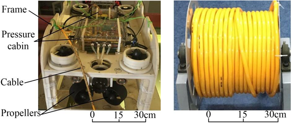
A prototype of ROV and a winch. ROV: remotely operated vehicle.

Structure and function of vehicle

In the previous research, many underwater vehicles had been developed. Liu et al.¹⁰ designed a new multifunctional and model-switched ROV for decomposition of an underwater structure at sea. Miao et al.²³ presented a small inspection-class underwater vehicle that carried a video camera for an underwater inspection. Anwar et al.²⁴ designed a portable low-cost ROV that conducted surveys in a shallow water. Pavol and colleagues^25
–27 designed an inertial navigation system applied to a mobile robot, which was benefit for an underwater navigation of a robot.

These previous vehicles were used only to observe in water, which can’t perform complex tasks. Most recently, we designed and manufactured an open-frame underwater vehicle for cracked walls of a nuclear power pool in emergency and a routine patrol inspection. The main parameters of a vehicle are shown in Table 1.

Table 1.

Main parameters of an underwater vehicle.

Symbol	Value	Remarks
L × B × H	1.06 × 0.65 × 0.66 m	Size of a vehicle
M	117 kg	Mass of a vehicle
V	0.21 m³	Volume of a vehicle

The vehicle system includes a frame, two pressure cabins, eight propellers, buoyancy material, a cable, a winch, and so on. A weld device was arranged on the vehicle to weld. The diameter of the cable, which can transfer signals and power for the vehicle and welding actuators, was 28 mm. And the cable was composed of outer sheath, armored, inner sheath, aluminum sheath, insulating layer, and cabling. The withdrawing and deployment was operated by a winch with a vehicle movement. The prototype of a vehicle and a winch is shown in Figure 1.

Theoretical modeling and solution

In general, there was a safe distance between a water surface and a pool shore in the vertical direction (z-axis) to ensure safety of a nuclear power pool in Figure 2. To describe the model precisely, a cable was divided into two parts: l₁ in water and l₂ in air. The intersection point P of a cable and the water surface was named as an entry water point, and the angle between a tangent line of an entry water point and the water surface was named as the entry water angle α. A fixed coordinate system o-xyz, which the origin was set on the water surface, and a local coordinate system b-t-n, which was attached on the cable, were established, and the t-axis was the tangential direction.

Figure 2.

A fixed coordinate system and a local coordinate system.

The cable attitude was depicted by the Euler angle θ and φ. The angle θ between the tangential projection of a cable and the x-axis was represented as an azimuth angle, and the angle φ between the tangent of a cable and x-o-y was an elevation angle. The water depth in the reactor was indicated as h; the distance between ROV and the pool bottom was h₀.

Then, a steady-state mechanical model of part l₁ was established, which was similar to part l₂. Here, the process of the steady-state mathematical modeling was described following the terminology of part l₁. The ratio of length to diameter was much bigger compared with a case of sea. The cable in the water was subjected to forces, including buoyancy, gravity, and resistance by surrounding flow, tension, the normal shear force, and normal moment, as shown in Figure 3.

Figure 3.

A schematic diagram of cable force microelement.

The steady-state equilibrium equation of the cable Microelement²⁸ can be expressed as

\frac{D F}{D s} + G + B + D = 0

where F = (T, S_b, S_n), T represents cable tension, S_n represents a shear force in the normal direction, S_b represents a shear force in the binormal direction, G represents the gravity of a cable, B represents the buoyancy, D represents the fluid resistance, and s represents the arc length.

The resultant force of gravity and buoyancy was called a restoring force W, which can be expressed as in a local coordinate system

\begin{array}{l} W = G + B = - m (g - ρ A) k \\ = - m (g - ρ A) sin φ t - m (g - ρ A) cos φ n \end{array}

where m is the mass per unit length, ρ is the density of fluid, and A is the cross-sectional area of the cable.

Therefore, the fluid resistance can be expressed as D in the local coordinate system

{\begin{array}{l} D_{t} = - \frac{1}{2} ρ d π \sqrt{1 + ε} C_{t} u_{t} | u_{t} | \\ D_{b} = - \frac{1}{2} ρ d \sqrt{1 + ε} C_{b} u_{b} \sqrt{u_{b}^{2} + u_{n}^{2}} \\ D_{n} = - \frac{1}{2} ρ d \sqrt{1 + ε} C_{n} u_{n} \sqrt{u_{n}^{2} + u_{b}^{2}} \end{array}

where u_t, u_b, and u_n are the tangential, binormal, and normal velocity of a cable Microelement, respectively; C_t, C_n, and C_b are the cable tangential coefficient, normal coefficient, and binormal coefficient, respectively; d represents a cable diameter; ε represents a cable strain and ε = T/(EA), E is an elastic modulus.

In the local coordinate system, the cable force F on space differential can be written as

\frac{D F}{D s} = \frac{\partial F}{\partial s} + Ω \times F

where Ω is the curvature of a cable at s. The binormal curvature and the normal curvature were respectively written as

Ω_{b} = \frac{d φ}{d s}

Ω_{n} = - cos φ \frac{d θ}{d s}

where Ω_b and Ω_n are a binormal curvature and a normal curvature, respectively.

According to equations (1) to (4), governing equations can be obtained in the local coordinate system as follows

\frac{d T}{d s} = S_{n} \frac{d φ}{d s} + S_{b} cos φ \frac{d θ}{d s} + g (m - ρ A) sin φ + \frac{1}{2} ρ π d \sqrt{1 + ε} u_{t} | u_{t} |

\frac{d S_{b}}{d s} = - T cos φ \frac{d θ}{d s} + S_{n} sin φ \frac{d θ}{d s} + \frac{1}{2} ρ d \sqrt{1 + ε} C_{n} u_{b} \sqrt{u_{n}^{2} + u_{b}^{2}}

\frac{d S_{n}}{d s} = - T \frac{d φ}{d s} - S_{b} sin φ \frac{d θ}{d s} + g (m - ρ A) cos φ + \frac{1}{2} ρ d \sqrt{1 + ε} C_{n} u_{n} \sqrt{u_{n}^{2} + u_{b}^{2}}

According to the moment balance equation of a cable, we can obtain after omitting higher order infinitesimal part

\frac{d M_{b}}{d s} = \frac{- M_{b}^{2} tan φ}{E I} - S_{n} {(1 + ε)}^{3}

\frac{d M_{n}}{d s} = \frac{M_{b} M_{n} tan φ}{E I} + S_{b} {(1 + ε)}^{3}

where M_b is the binormal moment, M_n is the normal moment, and the moment of inertia of a cable is I.

The differential relation between a fixed coordinate system and a local coordinate system is

{\begin{array}{l} \frac{d x}{d s} = (1 + ε) cos φ cos θ \\ \frac{d y}{d s} = (1 + ε) cos φ sin θ \\ \frac{d z}{d s} = (1 + ε) sin φ \end{array}

The steady-state mathematical model of the cable l₁ was the same as that of the cable l₂. The difference was the medium density in which the cable laid.

Therefore, the steady-state governing equation set of the part l₁ was composed of formula (5) to (12). The unknowns to be solved were T, S_b, S_n, Ω_b, Ω_n, x, y, z, θ, and φ. An initial condition, which was a state value of an endpoint or any point of a cable, was needed to obtain the numerical solution. The problem of solving ODE set was transformed into an initial value problem, which was a key to get an initial value. For the part l₁, a vehicle was always connected with the cable, a state value of the connection point can be obtained according to a motion state. On the basis of the transformation between a fixed coordinate system and a local coordinate system, the initial force value of the connection point was

{\begin{array}{l} T_{0} = sin θ_{0} cos φ_{0} F_{x} + cos θ_{0} cos φ_{0} F_{y} + sin φ_{0} F_{z} \\ S_{b 0} = cos θ_{0} F_{x} - sin θ_{0} F_{y} \\ S_{n 0} = - sin θ_{0} sin φ_{0} F_{x} - cos θ_{0} sin φ_{0} F_{y} + cos φ_{0} F_{z} \end{array}

where F_x, F_y, and F_z are the external forces on the vehicle which can be calculated by computational fluid dynamics (CFD).^29
–31 T₀, S_b0, and S_n0 are the initial value of the tension, binormal force, and normal force, respectively.

The initial value of an azimuth angle θ₀ was the angle between the motion direction of a vehicle and the y-axis, and the initial value of the elevation angle φ₀ was equal to the entry water angle α. A cable was connected to the vehicle through a hinge; hence, the initial value M_b0 and M_n0 can be set as 0.

The part l₂ of a cable was connected with a part l₁ by the entry water point P. They were coupling, namely, the point P was the upper endpoint of l₁, and was synchronously the lower endpoint of l₂. The state value of point P can be obtained by solving ODE set of the part l₁, which was considered as the initial value of the governing equation set of l₂.

The initial value problem was solved by the fourth Runge–Kutta algorithm which was crucial for the size of an iterative step, and the step size should be set in theory to obtain a fine accuracy. While the cable length was often tens of meters or even longer in practice, which can result in hundreds of numbers of iterative steps. If the step size was larger, the results got harder to converge. Here, to balance the relationship between accuracy and computing efficiency, the steady-state governing equations of the cable were dimensionless treatment, namely the length which was actually tens of meters was consider as 1.0. The unknowns in the governing equation set were dimensionless as given in Table 2.

Table 2.

The correlation of standard unit and dimensional coefficients.

Standard unit, Q	Dimensional coefficient, q	Remarks
s	l	Arc length
X	l	Position coordinate
V	$\sqrt{g l}$	Velocity
F	mgl	Cable force
M	$m g l^{2}$	Cable moment
W	mg	Restoring force

Where l is the length of a cable, and we defined

q_{n} = \frac{Q}{q}

The formula was defined as follows

α_{1} = \frac{m g l}{E A}, α_{2} = \frac{m g l^{3}}{E I}, γ = \frac{ρ d l}{m}

According to Table 2, formulas (14) and (15) the governing equation set (5) to (12) can be dimensionless treatment, and then a dimensionless steady-state governing equation set can be obtained.

Environmental factors analysis

Most of the work was done when an underwater vehicle was in a steady state. We picked the tension T, the normal shear force S_n, and the binormal moment M_b to investigate the steady-state mechanical characteristics of a cable, which was directly related to the vehicle velocity, the water depth, the entry water angle, density, cable length, and so on. The underwater vehicle (Figure 2) moved along the y-axis in line; hence, the direction angle θ₀ was set to be 0° consistently. The position of a winch on the shore was set as (x, y, z) _N = (0, 0, 0). The physical characteristics of the cable are given in Table 3.

Table 3.

The physical characteristic of the cable.

Symbol	Value	Remarks
d	0.028 m	Diameter of the cable
m	0.95 kg/m	Mass per length
C _n	1.44	Normal coefficient
C _b	1.44	Binormal coefficient
C _t	0.15	Tangential coefficient
E	2E11 Pa	Elasticity modular
p_v	0.5	Poisson ratio

Velocity influence on the steady-state mechanics

The resistance of a vehicle which moved uniformly in line was calculated by CFD. The state value of a connection point was obtained by formula (13). Here, the velocity was, respectively, set as v = −0.1, −0.2, −0.3, and −0.4 m/s. And, other condition was that the water depth was 20 m, the entry water degree was 30°, and the cable length was 30 m. Through calculating the tension T, the normal shear force S_n, the binormal moment M_b could be respectively obtained under v = −0.1 to −0.4 m/s, the results were shown as Figure 4.

Figure 4.

The influence of a vehicle motion on the steady-state mechanics. The effect on (a) tension, T, (b) normal force, S_n, (c) binormal moment, M_b, and (d) the steady-state configuration.

The tension T shown in Figure 4(a) increased obviously at the same position of the cable as the vehicle velocity increased, and there was a linear relationship between arc length and the tension in water or in air; due to medium change, the gradient in water was less than that in air. Although an initial value of the normal shear force S_n decreased with an increase in velocity, there was little influence in Figure 4(b). From Figure 4(c), we can find that there was a decreasing curve between arc length and the binormal moment S_b with an increase in the velocity, and the curvature was unchanged at the entry water point. From Figure 4(d), it can be found there is no detectable influence on the steady-state configuration of a cable in the z-axis direction.

Water depth influence on the mechanics

The water temperature can rise as the nuclear fuel rods were cooled in the pool. Then, the water depth fell due to the evaporation, which can result in decreasing the length of the part l₁. When the velocity was v = −0.2 m/s, the results under the condition of water depth 16, 18, 20, and 21 m are shown in Figure 5.

Figure 5.

The influence of water depth on the steady-state mechanics. The effect on (a) tension, T, (b) normal force, S_n, (c) binormal moment, M_b, and (d) the steady-state configuration.

From Figure 5(a), it can be obtained that the tension T of the upper point (i.e. the connection point between a winch and a cable) substantially increased as the water depth decreased, and there was no influence on the tension of the part l₁. From Figure 5(b), it can be found that there was an obvious increase in the normal shear force S_n with the decrease in the water depth, and the change trend was similar to that of tension. In Figure 5(c), a curve between arc length and the binormal moment M_b is shown, and the less the depth was, the more the binormal moment of the upper point was. In Figure 5(d), there was no detectable influence on the steady-state configuration of a cable in the z-axis direction.

Entry water degree influence on the mechanics

The entry water degree changed with the position of a vehicle in the pool, which can result in the length change of the part l₁ and the part l₂ and the position change of an entry water point. Here, an entry water degree was set as 20°, 25°, 30°, and 35°. The velocity was v = −0.2 m/s, and the water depth was 20 m. The effect of an entry water depth on the steady-state mechanical properties is shown in Figure 6.

Figure 6.

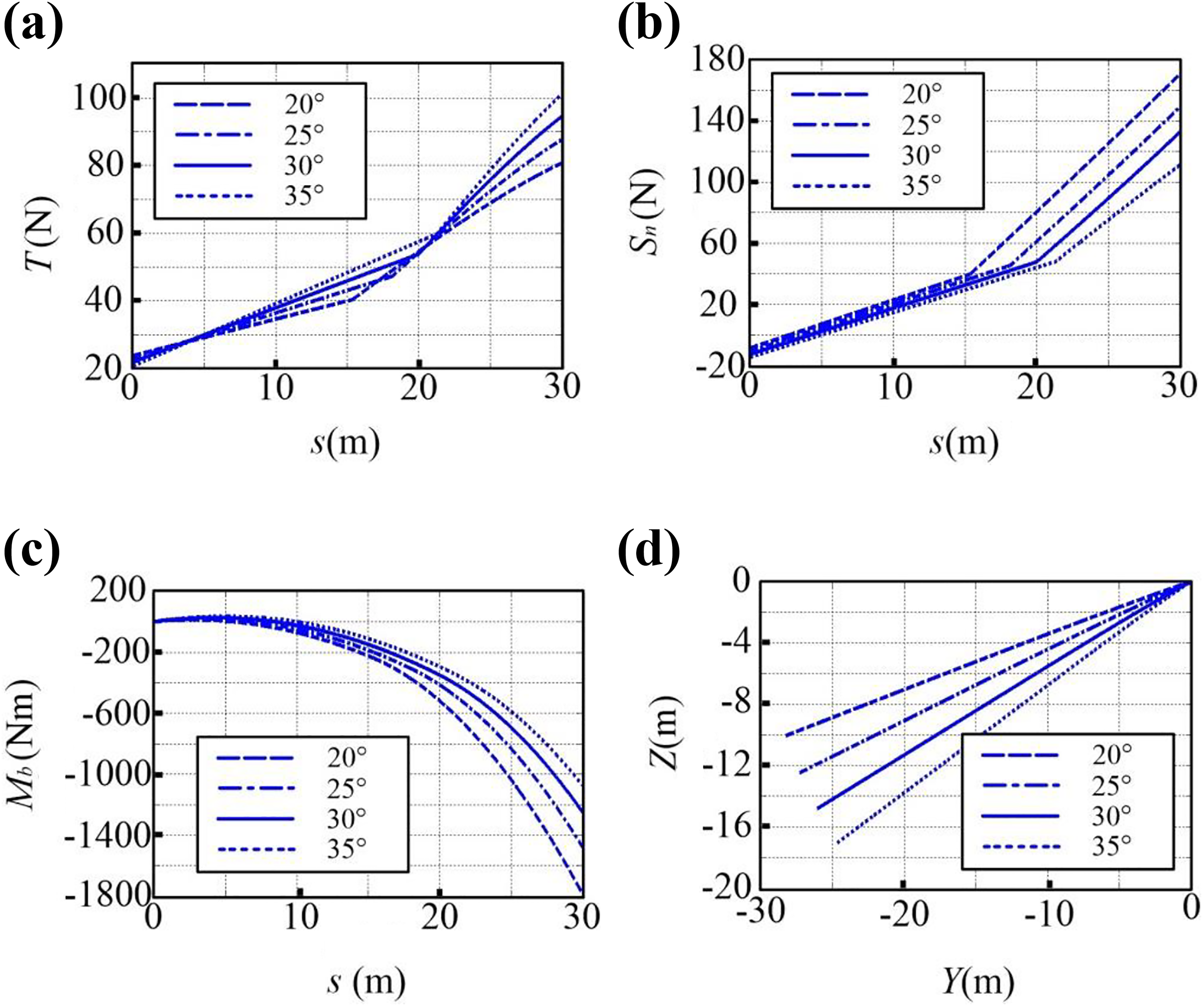
The influence of the entry water angle on the steady-state. The effect on (a) tension, T, (b) normal force, S_n, (c) binormal moment, M_b, and (d) the steady-state configuration.

From Figure 6(a), it was found that the tension T of the upper point increased obviously with an increase of the entry water angle, and there was a linear trend for the tension of the part l₁ and l₂. From Figure 6(b), we knew that the normal shear force S_n was markedly decreased when the entry water angle changed from 20° to 35°, and the linear trend was closed to that of the tension. In Figure 6(c), the binormal moment M_b was reduced with the increase in the angle. In Figure 6(d), it can be found that the more the entry water angle was, the more the depth of the lower endpoint was in the z-axis direction.

Water density influence on the mechanics

The water in the pool which contained 2000–2500 ppm boric acid was faintly acid. The density and concentration of water can increase with an increase of water temperature. The water density had an effect on the steady mechanical properties of the cable. Here, the water density was set as 1006, 1015, 1030, and 1040 kg/m³. The results of the tension T, the normal shear force S_n, and the binormal moment S_b are shown in Figure 7.

Figure 7.

The influence of density on the steady-state mechanics. The effect on (a) tension, T, (b) normal force, S_n, (c) binormal moment, M_b, and (d) the steady-state configuration.

From Figure 7(a), it can be found the tension T at the same position of the cable had a tiny decrease with a density increase, and the linear trend was always kept. In Figure 7(b), there was a little decrease in the normal shear force S_n due to the density change from 1006 kg/m³ to 1040 kg/m³. From Figure 7(c), it can be found that the binormal moment M_b was reduced when the density increased. In Figure 7(d), there is little influence on the steady-state configuration due to density change.

Cable length influence on the mechanics

When the vehicle moved uniformly in a line, the cable length can vary with a withdraw and deployment of a winch. At meantime, the entry water angle and the length of the part l₁ and l₂ also altered. Here, the velocity was −0.2 m/s in the y-axis direction. With an increase in the length of the cable, the tension T, the normal shear force S_n, and the binormal moment M_b of the upper point are shown in Figure 8.

Figure 8.

The influence of the length of cable on the steady-state mechanics. The effect on (a) tension, T, (b) normal force, S_n, and (c) binormal moment, M_b.

From Figure 8(a), we can find that with an increase in the length of the cable, the tension T of the upper point decreased linearly, but the scale was very small. Figure 8(b) showed that there was a liner increase in the normal shear force S_n with the increase in length. In Figure 8(c), the binormal moment M_b increased linearly, and the amplitude of growth was large.

A test of a cable mechanics

It is almost impossible to carry out a full-scale experiment of a cable mechanics due to dozens of meters of the cable long on the tail of a vehicle. At present, the mechanics experiment of underwater cables was very limited, most of which was a resistance measurement. In this section, the mechanical properties of the cable arranged on the vehicle were measured by a self-made experimental model and a dynamic signal analyzer in a circulating tank, which can prove the correctness of the cable mechanical model and the validity of the numerical solution.

The test design of a cable mechanism

The test platform of a cable mechanism consisted of a data acquisition system which can monitor real-time change of a cable mechanism and the flow velocity of a circulating tank by a dynamic signal analyzer and a self-made experiment model with a strain gauge sensor which was arranged on the fixed frame of a circulating tank. The test platform is shown in Figure 9.

Figure 9.

A test platform of a cable force. (a) A data acquisition system and (b) the underwater experiment model.

It is a key for this to make a self-made cable model in this test, which consisted of a physical model, a strain sensor, and an elastic base. A section of the cable on the vehicle which was 2.5 m long was treated as a physical model, and four sets of strain gauge sensors were distributed equally on the model. The distance from the free end of a cable was 0.3 m (observation point no. 1), 0.85 m (observation point no. 2), 1.4 m (observation point no. 3), and 1.95 m (observation point no. 4), respectively. At every observation point, there were four strain gauge sensors uniformly arranged in the circumference. The chip and the lead connection of a sensor were sprayed with insulating paint, which had an effect of sealing and waterproofing. The physical model of the cable and the arrangement of a strain gauge sensor are shown in Figure 10.

Figure 10.

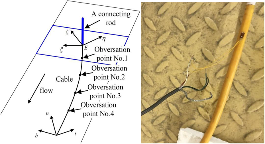
The physical model of a cable.

According to the vehicle operation, the flow velocity in a circulating tank was set as 0.35, 0.45, and 0.55 m/s, respectively, which can prevent a cable rising to the water surface due to the excessive flow velocity and the deformation of a sensor suppressed due to the small flow velocity. The tension of each point was 0–15 N under the flow velocity 0.35–0.55 m/s based on the previous research,^32
–34 which required a sensor selected with a suitable range, a high measuring accuracy, and a small size of sensitive grating. Based on all above mentioned requirements, the specification of a strain gauge sensor selected was BFH120-3AA-D100, and the technical indexes are given in Table 4.

Table 4.

The indexes of a sensor BFH120-3AA-D100.

Electric resistance	Sensitivity coefficient	Chip size	Sensitive grid size
120 Ω	2.0 ± 1%	6.9 × 3.9 mm²	3.0 × 2.3 mm²

The elastic base was an important component of a strain sensor, and the selection of material followed the principles: the base produced a large deformation under a small force with a good linearity; the base was easily processed to make the shape required for testing; and the base was hard to react chemically with the cable skin with a good adhesion. Through repeated experiments, the phenolic resin was selected as the elastic base material.

To obtain the relationship between the mass and a strain, the sensor was statically calibrated, that is, the strain was obtained by a dynamic signal analyzer due to the gravity from a weight loaded on the sensor. Then, a function between mass and strain was got. The test platform of a strain gauge sensor calibration is shown in Figure 11.

Figure 11.

A test platform of a strain gauge sensor calibration.

The weights, which were 100, 200, 300, 400, 500, 700, 1000, and 1500 g, respectively, were loaded at the end of a cable to calibrate a strain gauge sensor. The strain values can be obtained as given in Table 5.

Table 5.

The strain values of sensors under different mass values.

Mass (g)	100	200	300	400	500	700	1000	1500
Strain (μm)	128.51	200.04	243.89	259.09	284.46	313.03	329.18	340.79

The relation between strain and mass can be gained by a data fitting

m_{F} = 3.931 \times 10^{- 12} e^{0.09582 μ} + 23.33 e^{0.01073 μ}

where m_F represents the mass of a weight and μ represents the strain.

The process and results of a test

In this section, the cable mechanism was under the flow velocity 0.35, 0.45, and 0.55 m/s. In every working condition, an acceleration of the flow lasted for 1 min, then a uniform movement continued for 1 min, and finally, the flow decelerated to a rest. The mean strain of three tests repeated was considered as the result by a dynamic signal analyzer.

When the flow acted on the cable, the deformation of a strain gauge on the cable can be measured by a dynamic signal analyzer to obtain the tension. Under the flow velocity 0.35, 0.45, and 0.55 m/s, the results of tension by a test and a simulation are shown in Figure 12.

Figure 12.

The comparison between test and simulation results of a cable tension at 0.35, 0.45, and 0.55 m/s. The tension under the flow velocity (a) 0.35 m/s, (b) 0.45 m/s, and (c) 0.55 m/s.

From Figure 12(a), we can find that the simulation results were larger than those by the test at all observation points, but the error was below 10%. In Figure 12(b), the error between the results from simulation and test was not more than 10% at the observation point no. 1, no. 2, and no. 3, and the error almost was 18% at the observation point no. 4. In Figure 12(c), the simulation results were closed to those by a test, in which error was below 5% at the observation point no. 1, no. 2, and no. 3, but at the observation point no. 4, the error was almost 17%. In summary, the error was acceptance, which verified the mechanical model of a cable and the simulation results.

Conclusion

In this work, the steady-state mechanical characteristic of a cable on the vehicle was studied. A theoretical model of the cable considering medium change was regarded as an ODE set solved, and then the effects of environment factors on steady-state mechanical properties were quantified. With a velocity increase from 0.1 m/s to 0.4 m/s, the tension and normal shear force at the upper point climbed at a rate of 35% and 5%. Also there was no influence on an initial state, but at the upper point, the binormal moment decreased by 10%. The water depth decreased from 21 m to 16 m; the tension, the normal force, and the binormal moment increased by 40%, but there was no influence for the vehicle position. With an increase of entry water angle from 20° to 35°, the tension grew by 43%, but the normal force and binormal moment decreased by 38% and 50%, respectively. The density had a tiny influence on cable force and moment decreased within 5%. With an increase in the length of cable, the tension decreased by 2.6%, but the normal force increased by15% and the binormal moment increased by 32%. By comparing the simulation with experimental results, the authenticity of the mechanical model of a cable was verified, and the numerical method was shown to be reasonable. The results demonstrated that the presented method can be used to evaluate the effect of real environment factors on a steady-state motion of a vehicle and held a potential to improve the mechanism design and control strategy. In the near future, the dynamic-state mechanical characteristic will be modeled, which are solved by simulation, and then the effects of environment factors and motion parameters on the mechanical properties will be quantified.

Footnotes

Declaration of conflicting interests

The author(s) declared no potential conflicts of interest with respect to the research, authorship, and/or publication of this article.

Funding

The author(s) disclosed receipt of the following financial support for the research, authorship, and/or publication of this article: The study was supported by the Self-Planned Task of State Key Laboratory of Robotics and System (HIT; No. SKLRS201804B) and the National Natural Science Foundation of China (No. 61673138).

ORCID iD

Zhan-Dong Li

Jian-Guo Tao

References

Zheng

Tagami

Uchida

. Release of plutonium isotopes into the environment from the Fukushima Daiichi nuclear power plant accident: what is known and what needs to be known. Environ Sci Technol 2013; 47(17): 9584–9595.

Cavoski

Revisiting the convention on nuclear safety: lessons learned from the Fukushima accident. Asian J Int Law 2013; 3(2): 365–391.

Ramadass

Ramesh

Selvakumar

. Deep-ocean exploration using remotely operated vehicle at gas hydrate site in Krishna–Godavari basin, Bay of Bengal. Curr Sci 2010; 99: 809–815.

Salgado

Gonzalez

Martinez

. Deep water ROV design for the Mexican oil industry. In: Oceans conference, Sydney, Australia, 24–27 May 2010, pp. 1–6. IEEE.

Park

Yeu

Yoon

. A study of sweeping coverage path planning method for deep-sea manganese nodule mining Robot. In: Oceans conference, Waikoloa, HI, USA, 19–22 September 2011, pp. 19–22. IEEE.

Nagatani

Kiribayashi

Okada

. Emergency response to the nuclear accident at the Fukushima Daiichi nuclear power plants using mobile rescue robots. J Field Robot 2013; 30(1): 44–63.

Dong

Wang

Xing

. Design and control of a tracked robot for search and rescue in nuclear power plant. In: International conference on advanced robotics & mechatronics, Macau, China, 18–20 August 2016, pp. 330–335. IEEE.

Zeng

Zhou

Zheng

. Advance of hazardous operation robot and its application in special equipment accident rescue. In: International conference on mechanical engineering and control systems, Wuhan, China, 1–4 December 2015, pp. 340–343. World Scientific Publishing.

Buckham

Nahon

Seto

. Dynamics and control of a towed underwater vehicle system, part I: model development. Ocean Eng 2003; 30(4): 453–470.

10.

Liu

Song

Liang

. Design and experiment of control system for underwater ocean engineering structure inspection and cleaning remotely operated vehicle. Frontier Computing 2016; 32(3): 865–879.

11.

Vedachalam

Ramesh

Subramanian

. Design and development of remotely operated vehicle for shallow waters and polar research. In: Underwater technology, Chennai, India, 23–25 February 2015, pp. 1–5. IEEE.

12.

Walton

Polachech

. Calculation of transient motion of submerged cables. Math Comput 1960; 14(69): 27–46.

13.

Ablow

Schechter

. Numerical simulation of undersea cable dynamics. Ocean Eng 1983; 10(6): 443–457.

14.

Milinazzo

Wilkie

Latchman

. An efficient algorithm for simulating the dynamics of towed cable systems. Ocean Eng 1987; 14: 513–526.

15.

Chiou

. Nonlinear hydrodynamic response of curved singly-connected cables. Corvallis: Oregon State University, 1989.

16.

De Zoysa

APK

. Steady-state analysis of undersea cables. Ocean Eng 1978; 5(3): 209–223.

17.

Friswell

. Steady-state analysis of underwater cables. J Waterw Port Coast Ocean Eng 1995; 121(2): 98–104.

18.

Leech

Tabarrok

. The cable geometry for a towed submersible. Int J Mech Sci 1995; 37(10): 1079–1087.

19.

Wang

. Motion simulation and simulation of towing system for ocean exploration. Shanghai: Shanghai Jiao Tong University, 2006.

20.

Wang

Huang

Deng

D H

. Steady state analysis of towed marine cables. J Shanghai Jiaotong Univ (Sci) 2008; 13(2): 239–244.

21.

Wang

Yan

Chen

. A new adaptive time-delay control scheme for cable-driven manipulators. IEEE Trans Ind Inform 2018; 15(6): 1–12.

22.

Wang

Yan

. Practical adaptive fractional-order nonsingular terminal sliding mode control for a cable-driven manipulator. Int J Robust Nonlinear Control 2018; 29(5): 1396–1417.

23.

Miao

Pang

Miao

. Development of a low-cost remotely operated vehicle for ocean exploration. In: Oceans conference, Washington, DC, USA, 19–22 October 2015, pp. 1–7. IEEE.

24.

Anwar

Mohsin

Iqbal

. Design and fabrication of an underwater remotely operated vehicle (single thruster configuration). In: International Bhurban conference on applied sciences and technology, Islamabad, Pakistan, 12–16 January 2016, pp. 547–553. IEEE.

25.

Pavol

. Automated detection type body and shape deformation for robotic welding line. Adv Intell Syst 2014; 240: 229–240.

26.

Pavol

. Control of a robotic arm on the principle of separate decision of an inertial navigation system. Appl Mech Mater 2014; 611: 611–617.

27.

Pivarciova

Pavol

Turygin

. Analysis of control and correction options of mobile robot trajectory by an inertial navigation system. Int J Adv Robot Syst 2018; 15(1): 1–15.

28.

Howell

. Investigation of the dynamics of low-tension cables. MIT 1992; 21(5): 546–548.

29.

Jagadeesh

Murali

Idichandy

. Experimental investigation of hydrodynamic force coefficients over AUV hull form. Ocean Eng 2009; 36(1): 113–118.

30.

Zhang

Maxwell

Gerber

. Simulation of the flow over axisymmetric submarine hulls in steady turning. Ocean Eng 2013; 57(1): 180−196.

31.

Praveen

Krishnakutty

. Study on the effect of body length on the hydrodynamic performance of an axi-symmetric underwater vehicle. Indian J Geo-Mar Sci 2013; 42(8): 1013−1022.

32.

Jung

Park

Koterayama

. A numerical and experimental study on dynamics of a towed low-tension cable. Appl Ocean Res 2003; 25(5): 289–299.

33.

Liu

Zhang

. Transient dynamic analysis of towed low-tension cable with experimental verification. J Ship Mech 2013; 17(3): 197–214.

34.

Kwon

Park

Jung

. A numerical analysis for the dynamic behavior of the umbilical cable of a deep-sea unmanned underwater vehicle. Journal of Ocean Engineering and Technology 2005; 19(3): 31–38.

Analysis of cable force on steady-state motion of remotely operated vehicle for reaction pool underwater welding

Abstract

Keywords

Introduction

Structure and function of vehicle

Theoretical modeling and solution

Environmental factors analysis

Velocity influence on the steady-state mechanics

Water depth influence on the mechanics

Entry water degree influence on the mechanics

Water density influence on the mechanics

Cable length influence on the mechanics

A test of a cable mechanics

The test design of a cable mechanism

The process and results of a test

Conclusion

Footnotes

Declaration of conflicting interests

Funding

ORCID iD

References