Sage Journals: Discover world-class research

Abstract

This work focuses on multi-objective scheduling problems of automated manufacturing systems. Such an automated manufacturing system has limited resources and flexibility of processing routes of jobs, and hence is prone to deadlock. Its scheduling problem includes both deadlock avoidance and performance optimization. A new Pareto-based genetic algorithm is proposed to solve multi-objective scheduling problems of automated manufacturing systems. In automated manufacturing systems, scheduling not only sets up a routing for each job but also provides a feasible sequence of job operations. Possible solutions are expressed as individuals containing information of processing routes and the operation sequence of all jobs. The feasibility of individuals is checked by the Petri net model of an automated manufacturing system and its deadlock controller, and infeasible individuals are amended into feasible ones. The proposed algorithm has been tested with different instances and compared to the modified non-dominated sorting genetic algorithm II. The experiment results show the feasibility and effectiveness of the proposed algorithm.

Keywords

Automated manufacturing system multi-objective optimization Petri net scheduling genetic algorithm

Introduction

Scheduling is a resource allocation process over a period of time to perform a set of tasks.¹ Flexible flow-shop and job-shop scheduling (FSP and FJS, respectively) are one of the most important problems in the area of production scheduling, and these are all well-known non-deterministic polynomial-time (NP)-hard.² In the study of these scheduling problems, it is usually assumed that the capacity of buffers for storing jobs is unlimited, and hence, when a machine has finished processing a job, the job can leave immediately, and the machine can start processing other jobs, that is to say, there is no blockage. However, in practical automated manufacturing systems (AMSs),^3–5 machines, buffers, robots, and other resources that can hold jobs are always limited. The finiteness of all these resources makes the system not only have the blockage problem but also encounter the so-called deadlock.^6–21 The deadlock situation occurs when a set of jobs are in “circular waiting,” that is, each job in the set waits for a resource held by another job in the same set.⁹ For such an AMS, the required resource allocation or scheduling strategy can not only prevent the system from falling into deadlock but also optimize the system performance.^{7,12,13,22–26} Therefore, it is more important to develop such a scheduling strategy.

In order to solve the problem of optimization scheduling for AMSs with limited resources, deadlock control strategies should be established in advance.²² This is much of the reason that the deadlock problem of AMSs has been studied extensively. Since Petri nets (PNs) can clearly describe the characteristics of AMSs such as resource sharing, conflict, concurrency, and deadlock,^14–18 they are widely used to model the dynamic evolution of AMSs. Based on PNs, various deadlock control strategies or controllers for AMSs have been proposed, mainly including two kinds: deadlock avoidance and deadlock prevention. Of these, the former are online control policies that use feedback information on the current resource allocation status and future process resource requirements to keep the system away from deadlock states,^13,14 while latter are offline and guarantee that necessary conditions for circular waiting or deadlock cannot be satisfied at any time of the AMS dynamic.^20–24

The joint consideration of scheduling and deadlock control of AMSs leads to more complex and difficult combinatorial optimization problems. Classical scheduling methods for flexible flow-shop and FJS cannot be directly used to solve such problems, while it is a great challenge to extend and modify them for deadlock-prone AMSs. Therefore, there are few researches on AMS scheduling. Ramaswamy and Joshi⁷ established a mathematical programming model of the scheduling problem for AMS with no route flexibility, and a Lagrangian relaxation heuristic was used to search for the optimized average flow time. Gomes et al.⁸ investigated the scheduling problem of flexible job-shop with groups of parallel homogeneous machines and limited intermediate buffers, and developed the integer linear programming model of the scheduling problem to meet the just-in-time due dates. By solving this integer linear programming, an optimal schedule can be obtained if it is feasible. Brucker et al.¹⁰ and Heitmann¹¹ investigated job-shop scheduling problems with limited buffer constraints by classifying buffers into machine-dependent output and input buffers, and part-dependent buffers. Fahmy et al.^12,13 presented an insertion heuristic based on Latin rectangles. This heuristic is capable to take into account limited buffer capacities and to avoid deadlocks, and hence, can obtain a feasible schedule.

In Xing et al.,²⁵ a genetic scheduling algorithm for AMSs is developed directly using a predesigned controller to minimize the makespan. Based on the deadlock search algorithm,²⁰ a one-step look-ahead method is developed to avoid deadlocks by amending those infeasible individuals to feasible ones. A feasible individual can be decoded directly to a schedule. This approach is improved in Han et al.²⁶ using different kinds of crossover and mutation operations in genetic algorithm. Computational results show the good improvement in performance. At the same time, based on the one-step look-ahead method presented in Xing et al.,²⁰ several kinds of heuristic and intelligence optimization scheduling algorithms are established.^27,28 Baruwa et al.²⁹ proposed a heuristic scheduling algorithm based on timed-colored PNs. During the exploration, deadlock states are marked and the paths to those states are terminated to prevent the system from encountering them.

All above research on scheduling problems of AMSs has been concentrated on single objective alone. However, several objectives must be considered simultaneously in the real-world production situation and these objectives often conflict with each other. Previous research on multi-objective scheduling mainly focused on flexible flow-shop and FJS,^30–39 while for deadlock-prone AMSs, it hardly involved. Kacem et al.³⁰ developed an effective evolutionary algorithm to solve multi-objective scheduling problems for flexible job-shops. An effective hybrid tabu search algorithm for solving multi-objective flexible job-shop scheduling problems was introduced by Li et al.³¹ A Pareto-based particle swarm optimization and local search approach to multi-objective scheduling problems of flexible job-shops was proposed by Moslehi and Mahnam.³² Rahmati et al.³³ proposed two evolutionary algorithms to solve the flexible job-shop scheduling problems with three objectives. To solve multi-objective flexible job-shop scheduling problem, a hybrid discrete particle swarm optimization algorithm with simulated annealing algorithm and Pareto-based grouping discrete harmony search algorithm were proposed by Shao et al.³⁴ and Gao et al.³⁵ For solving the multi-objective flexible job-shop scheduling problem with limited resource constraints, a hybrid discrete firefly algorithm is presented in Karthikeyan et al.,³⁶ where limited resource constraints are used to balance between the resource limitation and machine flexibility. While for different multi-objective flow-shop scheduling problems, many methods are proposed, such as estimation of distribution algorithm,³⁷ multi-phase covering Pareto-optimal front method,³⁸ and multi-phase approach.³⁹

For a multi-objective optimization problem, there is often no single optimal solution, but rather a set of optimal solutions, called as Pareto-optimal solutions. They are optimal in the wider sense that no other solutions in the search space are superior to them when all objectives are considered. A number of evolutionary algorithms have been used to deal with multi-objective optimization problems.^40,41 They generate widely different Pareto-optimal solutions by combination of parent and offspring populations and using various diversity-preserving mechanisms, and have the ability to find multiple Pareto-optimal solutions in one single run. The non-dominated sorting genetic algorithm II (NSGAII)⁴² is one of such evolutionary algorithms that is modified from non-dominated sorting genetic algorithms (NSGA) in Srinivas and Deb⁴⁰ and Deb⁴¹ and hence better than NSGA.

This article considers the multi-objective scheduling problems for deadlock-prone AMSs. A Pareto genetic algorithm (PGA) is proposed based on the PN models of AMSs. In the proposed PGA, a candidate schedule is first represented as an individual. Due to the constraint of limited resource capacity, these individuals in a population may be infeasible, that is, they cannot be directly decoded into feasible schedules or feasible firing sequences of transitions in PN model, and hence, it is necessary to check the feasibility of new individuals generated in initialization and genetic operators and modify infeasible individuals into feasible ones. In this article, deadlock control policies are used directly to check the feasibility of individuals and modify them if necessary, and the Pareto dominance and crowding distance in Shao et al.³⁷ are used to update solutions in the sense of multi-objective optimization, while a new elitist strategy in order to avoid premature convergence is proposed.

A set of simulation examples is used to show the feasibility and effectiveness of the proposed method. At the same time, the proposed algorithm is compared with NSGAII. Note that the basic NSGAII in Deb et al.⁴² is aimed at continuous optimization problems and cannot be directly used to solve our scheduling problems. In order to solve our combinatorial optimization problem, the basic NSGAII is modified first. In the modified NSGAII (MNSGAII), the mechanism of evolution and elitist strategy in the basic NSGAII is adopted directly, while a deadlock prevention policy is embedded to ensure individual feasibility. Hence, MNSGAII is actually another new algorithm for solving the multi-objective scheduling problem of deadlock-prone AMSs. The simulation results show that PGA and MNSGAII are feasible for solving the multi-objective scheduling problem considered, and PGA has better performance.

The remaining contents are organized as follows. In section “Modeling of AMSs and deadlock controller based on PNs,” PN scheduling modeling of AMS and its deadlock control policy are briefly reviewed. In section “Multi-objective deadlock-free genetic scheduling algorithm for AMSs,” the PGA is proposed. Section “Simulation results and comparisons” presents the results of the simulation computation and comparison. Section “Conclusion” concludes this article.

Modeling of AMSs and deadlock controller based on PNs

This section introduces the AMSs considered, and their PN scheduling models, and then the deadlock control policy used in this article.

PN scheduling models of AMSs

An ordinary PN is a four-tuple N = (P, T, F, M₀), where P and T are finite sets of places and transitions, respectively. F⊆ (P×T) ∪ (T×P) is the set of directed arcs. M₀ is the initial marking of N and M₀: P→ℤ⁺, where ℤ⁺ is the set of non-negative integers.

For place p ∈ P and transition t ∈ T, let ^•p (p^•) denote the set of input (or output) transitions of p, and let ^•t (t^•) denote the set of input (or output) places of t.

Transition t is enabled at M₀, if ∀p ∈ ^•t, M₀(p) > 0. An enabled transition t at M₀ can fire, resulting a new marking M, denoted by M₀[t > M, where M is obtained by removing one token from each input place of t and putting one token to each output place of t. Let R(N, M₀) be the set of all markings of N reachable from M₀.

The AMS considered in this article consists of m types of resources and can process n types of jobs. A type of resources may be some identical machines, robots, automatic guidance vehicles, and buffers. The capacity of each type of resources is limited.

A job can have multiple predefined sequences of operations and can be completed by processing all operations of such one sequence in order. The processing of an operation requires a unit resource and appropriate time. At the same moment, each unit resource can process at most one job, and a job can only be processed on one unit resource. We assume that the resources for processing two adjacent operations in the same sequence are different, and all jobs and resources are available at the beginning. For job j, let O_j = o_j₁o_u₂…o_jL_(j) be a predefined operation sequence for it, and ℜ(o_jk) be the resource required for processing operation o_jk. Then, ℜ(O_j) ≡ℜ(o_j₁)ℜ(o_j₂) …ℜ(o_jL_(j)) is a processing route of job j though the system. The same type of jobs has the same set of processing routes.

Following the PN modeling methods proposed in Ezpeleta et al.²¹ and Xing et al.,²⁵ this article develops a PN model for AMS, called PN for Scheduling (PNS). The PNS of a simple flexible manufacturing system (FMS) is depicted in Figure 1.

Figure 1.

The PNS of a simple FMS.

In the PNS of an AMS, there are two classes of places, operation and resource places. A token in an operation place represents a job whose operation is being performed, while a token in a resource place represents that a unit resource is available. Resource type r is modeled by a resource place, denoted also as r. Its initial marking is the capacity of r, C(r), indicating that the maximum number of jobs that such type of resources can simultaneously hold.

A processing route or an operation sequence of a job is modeled by a path of transitions and operation places in PNS. For example, a predefined operation sequence of job j, O_j = o_j₁o_j₂…o_jL_(j) is modeled by a path π_j = t_j₁p_j₁t_j₂p_u₂…t_jL_(j)p_jL_(j)t_j_(L(j)+1), where place p_jk simulates operation o_jk of job j being processed on R(o_jk); the firing of a transition represents either the start or/and completion of an operation process, and the completion transition of the current operation is the same as the start transition of the next operation. For example, in Figure 1, t_j₁ is the start transition of operation o_j₁, while t_j₂ is the start transition of operation o_j₂ and the completion transition of o_j₁.

Two types of virtual places in PNS are used to model two classes of infinite buffers storing unprocessed and finished jobs, respectively. For example, in PNS shown in Figure 1, p_1s and p_2s store unprocessed jobs, and p_1e and p_2e store finished jobs of types, q₁ and q₂, respectively. The requirement and release of resources are modeled by arcs. If an operation o_ij modeled by place p in path π requires resource r, then add an arc from resource place r to start transition t₁ of o_ij and an arc from its completion transition t₂ to r. Then, for a given transition t, ^•t = ^(o)t ∪ ^(r)t, where ^(o)t is the input operation place of t and ^(r)t is the input resource place of t.

In addition, the processing time of an operation of a job is represented by time delay associated with the corresponding operation place, say p, and is defined as d(p). That is, PNS is a place-timed PN.

At the beginning, all jobs are unprocessed and the resources are idle and available. Then, the initial marking M₀ of PNS is M₀(p_is) = χ_i and M₀(r) = C(r), where χ_i is the number of type-q_i jobs and C(r) is the capacity of type-r resources; the initial markings of other places are 0. When all operations of all jobs are finished, tokens in p_is are moved into p_ie, and the PNS reaches its final marking M_f.

Example 1

Consider an AMS consisting of five machines m₁–m₅. Their capacities are given as C(m_i) = 1, i ∈ {1, 2, 4}, and C(m_j) = 2, j ∈ {3, 5}. The system can process two types of jobs, types q₁ and q₂. Type-q₁ jobs have two processing routes, denoted as w₁ and w₂, respectively. Type-q₂ jobs have one processing route, denoted as w₃. If three type-q₁ and two type-q₂ jobs are processed, then the PNS of the system is as shown in Figure 1, and there are three and two tokens in places p_1s and p_2s, respectively. Three processing routes for jobs are modeled by three paths in PNS, w₁ = p₁_st₁₁p₁₁t₁₂p₁₂t₁₃p₁₃t₁₄p₁₄t₁₅p_1e, w₂=p₁_st₁₁p₁₁t₂₂p₂₂t₂₃p₂₃t₂₄p₁₄t₁₅p_1e, and w₃ = p₂_st₃₁p₃₁t₃₂p₃₂t₃₃p₃₃t₃₄p_2e, respectively. At the beginning, the system state, that is, the initial marking of the PNS is M₀ = 3p_1s + 2p_2s + 2 m₁ + m₂ + m₃ + 2 m₄ + m₅, where kp denotes that place p has k tokens. When all the jobs are finished, the PNS reaches the final marking M_f = 2 m₁ + m₂ + m₃ + 2 m₄ + m₅ + 3p_1e + 2p_2e.

Deadlock controllers for PNS

Since all resources are finite, the considered AMS may enter deadlock state if not be properly constrained or controlled. A lot of research has been done on deadlock problem in AMSs and many deadlock prevention policies or controllers for AMSs have been proposed. All these policies can be directly used to avoid deadlock in stochastic Petri nets (SPNs). For details of the deadlock control, please refer to previous studies.^12–20

Multi-objective deadlock-free genetic scheduling algorithm for AMSs

Multi-objective optimization problem

In mathematical terms, a multi-objective optimization problem can be formulated as

\min F (x) = \min [f_{1} (x), \dots, f_{L} (x)] x \in X

where x is a feasible solution, F is a vector of L objective functions, and X is the feasible solution space. In a multi-objective optimization, there does not typically exist a feasible solution that optimizes all objective functions simultaneously. Therefore, attention is paid to Pareto-optimal solutions. That is, solutions that cannot be improved in any of the objectives without degrading at least one of the other objectives:

Pareto dominance: let x₁ and x₂ be two feasible solutions. x₁ is said to dominate x₂, denoted as x₁ ≺ x₂, if f_j(x₁) ≤ f_j(x₂), ∀j ∈ ℤ_L ≡ {1, 2, …, L} and ∃k ∈ ℤ_L, f_k(x₁) < f_k(x₂).

Pareto-optimal solution: a feasible solution x^* is a Pareto-optimal solution if there does not exist any other feasible solution which dominates x^*. The corresponding objective function is called the Pareto-optimal front vector f(x^*). The Pareto set is the set of all Pareto-optimal solutions and the corresponding objective vectors form the Pareto-optimal front.

Formulation of scheduling problem

Suppose that there are n jobs J₁–J_n to be processed, and the due date of J_i is d_i. The goal is to find a feasible schedule so as to optimize a set of predefined objectives. Such a feasible schedule is equivalent to a feasible sequence of firing transitions of the SPN model from the initial marking M₀ to final marking M_f.

For a feasible schedule π, let C_i(π) denote the completion time of job J_i under π, and the lateness of J_i is L_i(π) = C_i(π) – d_i. The following scheduling objectives are frequently used:^1,33,39

1. Makespan (C_max): it is the maximal of completion time of all jobs and can be defined as

C_{\max} = \max {C_{i} (p), i \in 1 Z_{n}}

2. Mean of earliness and tardiness (ϖ): it is the average of the earliness or tardiness of all jobs relative to their own due dates, denoted as

ϖ = \sum_{i \in 1 Z n} | C_{i} (π) - d_{i} | / n

3. Mean completion time (Δ): it is defined as Δ = Σ_{i ∈ ℤ}_n C_i(π)/n.

In this article, we consider the above three scheduling objectives—C_max, ϖ, and Δ. In PNS, let π = t₀t₁t₂…t_N₋₁ be a feasible sequence of transitions, o_ij denote the jth operation of J_i, and L(t_k[o_ij]) denote the earliest firing time of t_k that is also the start processing time of operation o_ij, where t_k[o_ij] denotes t_k as the start transition of o_ij. Feasibility of π implies that π can be fired sequentially. Thus, t_k[o_ij] can be fired only after operation o_i_(j−1) is finished and t_k₋₁ is fired. Let t_k₋₁ and t_s be the start transitions of o_uv and o_i_(j−1), respectively. The completion time of o_i_(j−1) is L(t_s[o_i_(j−1)])+d (o_i_(j−1)), and the firing time of t_k₋₁ is L(t_k₋₁[o_uv]). Then, L(t_k[o_ij]) = max{L(t_s[o_i_(j−1)]) + d(o_i_(j−1)), L(t_k₋₁[o_uv])}. The completion time of job J_i and the makespan of π are C_i(π) = max_j{L(t_k[o_ij]) + d(o_ij)} and C_max(π) = max_i, _j{L(t_k[o_ij]) + d(o_ij)}, respectively. Clearly, when due date d_i (i ∈ ℤ_n) is given, we can calculate ϖ and Δ based on C_i(α(π)).

Multi-objective scheduling algorithm

In order to obtain a feasible sequence of firing transitions to optimize multiple objectives, this article proposes a PGA based on PNS. In AMSs, a job may have multiple processing routes, and a scheduling should arrange not only a processing route for each job but also the start processing time of each operation. Hence, in the proposed PGA, an individual consists of two sections, route, and operation sections. The former sets up a processing route for each job, while the latter provides a sequence of operations of all jobs. As long as this operation sequence can be executed according to the given routes, this individual can be decoded directly into a feasible schedule, which is a feasible sequence of transitions without leading to deadlocks, and hence it is called as a feasible individual. Note that not all individuals are feasible because deadlocks may occur. With the help of the SPN model and its deadlock controller, the feasibility of each individual is checked and unfeasible individual is repaired to feasible one. The main components of the proposed PGA can be described in detail as follows:

1. Encoding and decoding: the encoding scheme in this work is based on the job permutation with repetition. A job permutation with repetition is a permutation of jobs, and each job may appear many times. Similar to Xing et al.,²⁵ an individual can be written as two sections π = (S_r; S_o), where S_r describes the route information of jobs and S_o is a permutation with repetition of all the jobs. S_r is an n-dimension vector S_r = (w₁, w₂, …, w_n), where n is the number of jobs and w_i represents the route through which job J_i is processed. In S_o, a type-x job J_i appears l(x) times, where l(x) is the number of operations on the longest processing route of type-x jobs.

In individual π = (S_r; S_o), let the jth J_i in S_o represent the jth operation of J_i on route w_i. Then, S_o can also be expressed as a sequence of operations (discarding redundant jobs), and by one-to-one correspondence between the operation and its start transition in PNS, π can be decoded uniquely as a sequence of transitions, denoted as α(π). In the decoding process, if there are some redundant J_i (i.e. the route specified by S_r for J_i, w_i, is shorter than the longest route of J_i), discard them.

Example 2

Reconsider the PNS shown in Figure 1. Now suppose that there are five jobs to be processed, three type-q₁ jobs J₁−J₃ and two type-q₂ jobs J₄−J₅. The PNS has three processing routes, denoted as w₁, w₂, and w₃, where w₁ and w₂ are for type-q₁ jobs and w₃ for type-q₂ jobs, respectively. Then, S_r₁ = (w₁, w₂, w₁, w₃, w₃) can be used as the first section of an individual π₁, meaning that jobs J₁−J₅ are processed through routes w₁, w₂, w₁, w₃, and w₃, respectively. Since l(q₁) = 4 and l(q₂) = 3, the operation section can be expressed as a permutation with repetition in which J₁, J₂, and J₃ all appear four times, while J₄ and J₅ appear three times, respectively. For example, S_o₁ = (J₁, J₁, J₅, J₃, J₂, J₂, J₄, J₅, J₂, J₃, J₃, J₄, J₄, J₅, J₂, J₁, J₁, J₃) can be used as the second section of π₁. Then, π₁ can be expressed as π₁ = (S_r₁; S_o₁) = (w₁, w₂, w₁, w₃, w₃; J₁, J₁, J₅, J₃, J₂, J₂, J₄, J₅, J₂, J₃, J₃, J₄, J₄, J₅, J₂, J₁, J₁, J₃). The first three terms of S_o₁ are J₁, J₁, and J₅, and represent the first and second operations of J₁ in route w₁, and the first operation of J₅ in route w₃, respectively. As a sequence of transitions, π₁ can be decoded as α(π₁) = (t₁₁[J₁], t₁₂[J₁], t₃₁[J₅], t₁₁[J₃], t₁₁[J₂], t₂₂[J₂], t₃₁[J₄], t₃₂[J₅], t₂₃[J₂], t₁₂[J₃], t₁₃[J₃], t₃₂[J₄], t₃₃[J₄], t₃₃[J₅], t₂₄[J₂], t₁₃[J₁], t₁₄[J₁], t₁₄[J₃]). Note that α(π₁) is not a complete and feasible sequence, that is, it cannot lead the system from M₀ to M_f, because it does not include the last transition in each route, say t₁₅ and t₃₄, and may lead deadlock. For completeness, add the last transition of each route for each job to the back of α(π₁), and α(π₁) added to these transitions is still denoted as α(π₁), called the transition sequence of π₁.

In the above decoding procedure, resource and deadlock control constraints are not considered. As a result, although α(π) contains complete firing transitions from M₀ to M_f, it may still be infeasible. Thus, the feasibility of each individual needs to be checked, and it is necessary to amend infeasible individuals into feasible ones.

2. Individual feasibility check and amendment: in this article, individual feasibility check and amendment is based on SPN and the used deadlock controller. When an individual is checked as infeasible, it is amended. The check and amendment are carried out in the same recursive procedure, and the details as shown in Algorithm IFCA.

Let (N, M₀) be the PNS model of an AMS and its deadlock controller (C, M_C). The controlled PNS can be expressed as (N_C, M_C₀) = (N, M₀) ⊗ (C, M_C). For a given individual π = (S_r; S_o) and its transition sequence α(π), the algorithm is a recursive procedure based on the controlled PNS (N_C, M_C₀). It begins from the first transition of α(π) and the initial marking M_C₀, and checks whether the current transition t is enabled at the current marking M. If t is enabled, update the current marking M by firing t and move to the next transition in α(π); otherwise, find the first enabled transition t* at M after t in α(π) and move t* to the tight front of t in α(π). If no transition after t is enabled at M, it is necessary to adjust the processing route of some job. Repeat the aforementioned steps until the last transition in α(π) is checked.

Since the controlled PNS is live, there exists at least one transition enabled at any reachable marking M ∈ R(N_C, M_C₀)\{M_f}. But, it is possible that none of transitions enabled at M are in the routes specified in π. That is, the routes that some jobs can take conflict with the specified ones. In this case, it is necessary to change the specified processing route in π for the corresponding job.

Algorithm IFCA: Individual feasibility check and amendment

Input: An individual π≡ (S_r; S_o);

Output: A feasible schedule α(π).

Generate π = (w₁, w₂, …, w_n; o₁, o₂, …, o_K) and α(π) = t₁t₂…t_K by decoding π;

Let i:= 1, and M_i:= M_C₀;

For (i = 1; i≤K; i ++) do {

For (j = 0; j < K; j++) do {

If (i + j ≤ N and t_i ₊ _j is enabled at M_i) then {

Set α(π) ≡t₁t₂…t_N := t₁t₂…t_i₋₁t_i ₊ _jt_i…t_i ₊ _j−1t_i ₊ _j ₊ ₁…t_K;

Set S_o≡o₁o₂…o_N:= o₁o₂…o_i₋₁o_i ₊ _jo_i…o_i ₊ _j−1o_i ₊ _j ₊ ₁…o_K;

M_i[t_i ₊ _j > M_i ₊ ₁;

break;

} //end If()

If (i + j > K) then { /*t_i, …, t_K are not enabledat M_i.*/

Find a transition t enabled at M_i. Suppose that the job enabling t is J_u, and t is on route w of J_u; //note that such t certainly exists, and w_u≠w.

Reset w_u = w, and update S_r, S_o, and α(π) correspondingly;

j = 0; /* restart from t_i.*/

} //end If()

} //end For(j)

} //end For(i)

Output α(π);

The individual feasibility checks and amendment in Algorithm IFCA are based on the controlled net, that is to say, the deadlock controller is designed beforehand. For a given individual, the number of transitions in α(π), K, is at most l * n, where l is the longest length of all processing routes and n is the number of jobs to be processed. That is, K≤l * n. The algorithm need to check all K transitions once, while for each of them, say t, at most all transitions after t in α(π), less than K transitions, are detected. Thus, at most K² transitions are detected in Algorithm IFCA, and hence, the algorithm has polynomial time complexity O((l * n)²).

When the algorithm is finished, a new feasible individual is obtained, and its corresponding sequence of transitions α(π) leads the PNS from M₀ to M_f, and hence, is feasible. If the algorithm does not adjust any order of transitions of the input sequence α(π), the input individual π itself is feasible.

3. Non-dominated sort and crowding distance: for a multi-objective optimization problem, generally, there is no single solution that is the best with respect to all objectives. Alternatively, there usually exists a set of non-dominated solutions or Pareto-optimal solutions, for which no improvement in any objective is possible without sacrificing at least one of the other objectives.

For a given population W, in order to identify solutions of its first non-dominated front F₁, Deb⁴¹ proposed a sorting algorithm, called as Fast-Non-Dominated-Sort, FNDS(W), in which each solution is compared with every other solution in W to find if it is dominated. The first front F₁ is a completely non-dominant set in the current population W, and actually, is the Pareto-front of W. Then, the algorithm is applied to the set of non–first front individuals, namely, W\F₁, and the second front F₂ is obtained. Repeat the algorithm, F₃, …, and F_V are computed. The algorithm sorts all individuals in population W into V non-dominated fronts F₁, F₂, …, and F_V, F_u ∩ F_v = ∅ for u ≠ v, and W = F₁ ∪ F₂ ∪ … ∪ F_V. The first front F₁ is a completely non-dominant set in W, the second front F₂ is dominated by the individuals in F₁ only, F₃ is dominated by the individuals in F₁ ∪ F₂, and so on. In this article, this Fast-Non-Dominated-Sort algorithm is used in the proposed PGA.

In the basic GA, the fitness function is used to guide simulations toward optimal solutions and the chromosome generation of the population. In this article, the individual fitness function is based on non-dominated fronts, and the fitness values of individuals in the same front are set to the same, and hence, for all individuals in F_k, their fitness values can be set to k. Thus, minimizing the fitness is the goal of simulation in this article.

Once the non-dominated sorting is completed, the crowding distance for individuals in front F_i can be calculated using the method proposed in Deb et al.⁴² and then used to estimate individual density in the population.

4. Genetic operations: once the individuals are sorted based on non-domination and with crowding distance assigned, every individual π_i in the population has two attributes, rank r_i and crowding distance d_i. Then, the selection is carried out using a crowded-comparison operator, denoted as ≺. Let π_i and π_j be two different individuals in the population. Define crowded-comparison operator as π_i ≺ π_j if r_i < r_j, or π_i ≺ π_j if r_i = r_j and d_i > d_j.

This means that for two individuals with different ranks, we prefer one with the lower rank, and one with the larger crowding distance for two individuals in the same front.

In this work, the tournament selection method is used in genetic operations. Two individuals are randomly chosen from the current population, and the better one is selected by the crowded-comparison operator as a parent individual for crossover. Repeat the process to select another parent individual.

Once the individuals for reproduction have been selected, the crossover and mutation genetic operators are applied to produce the offspring. The crossover operator applies to pairs of individuals, while the mutation operator applies to single individual. The goal of the former is to obtain better individuals by exchanging information in parent individuals. In this article, crossover is only done in the second section of individuals and Generalization of Order Crossover (GOX) is used. In the following, an example is used to describe its procedure. Reconsider the PNS in Example 1 and let π₁ and π₂ be two parent individuals:

π₁ = (S_r₁; S_o₁) = (w₁, w₂, w₂, w₃, w₃; J₁, J₁, J₅, J₃, J₂, J₂, J₄, J₅, J₂, J₃, J₃, J₄, J₄, J₅, J₂, J₁, J₁, J₃).

π₂ = (S_r₂; S_o₂) = (w₂, w₁, w₂, w₃, w₃; J₂, J₄, J₂, J₁, J₅, J₂, J₂, J₁, J₃, J ₁ , J ₄ , J ₅ , J ₃ , J ₄ , J ₃ , J₅, J₁, J₃).

π₂ is used as the donator of a crossover string. First, the crossover string is randomly chosen from the operation section of π₂. Second, all genes in π₁ that occur in the crossover string with the same operations are marked and then deleted. Finally, the crossover string is implanted into π₁ in the same position as it is in π₂.

Suppose that the length of crossover string in π₂ is 5, and the first gene of crossover string corresponds to o₁₃ or the third J₁ in S_o₂. In other words, the crossover string is σ = (J₁, J₄, J₅, J₃, J₄), and its corresponding operation sequence is (o₁₃, o₄₂, o₅₂, o₃₂, o₄₃). Next, delete jobs that correspond to operations o₁₃, o₄₂, o₅₂, o₃₂, and o₄₃ from π₁ and implant σ into S_o₁. Then, a new individual π₃ = (S_r₃; S_o₃) = (w₁, w₂, w₂, w₃, w₃; J₁, J₁, J₅, J₃, J₂, J₂, J₄, J₂, J₃, J ₁ , J ₄ , J ₅ , J ₃ , J ₄ , J₅, J₂, J₁, J₃) is obtained. Figure 2 shows this procedure of GOX with parents π₁ and π₂, where J_k is denoted as k for convenience.

Figure 2.

Illustration of GOX.

In order to increase the diversity of the population, the mutation operator further operates on a parent individual, generating a new offspring. Since an individual π = (S_r; S_o) includes route section S_r and operation section S_o, the mutation operator considers both two sections of an individual. First, another route (if any) can be reset for a job. For instance, in Example 1, type-q₁ jobs J₁, J₂, and J₃ have two routes w₁ and w₂, and thus their routes can be mutated between w₁ and w₂. While type-q₂ jobs J₄ and J₅ have only one route, and thus their routes cannot be mutated. For the mutation of S_o, the inversion mutation is adopted. In other words, we can select randomly a mutation string in S_o and then reverse it. Taking π₃ for example, we select a mutation string from the third to the eighth genes, that is, J ₅ , J ₃ , J ₂ , J ₂ , J ₄ , J ₂ , in S_o₃, and then obtain a new operation section S_o₃′ = (J₁, J₁, J ₂ , J ₄ , J ₂ , J ₂ , J ₃ , J ₅ , J₁, J₄, J₅, J₃, J₄, J₃, J₅, J₂, J₁, J₃) by reversing the selected string.

5. Elitist strategy: in the elitist strategy of the basic NSGAII, elite individuals in offspring and parent populations are effectively retained to the next population, and hence avoid optimal solutions from being lost in the evolutionary process. This evolutionary process may make all individuals in the first few non-dominant fronts of the population as elites, and may cause early convergence or convergence to local optima. For this reason, a new elitist strategy is proposed by improving one in the basic NSGAII in this article.

In our proposed elitist strategy, the offspring population is first combined with its parent population, forming a new combined population. Then, the combined population is sorted based on non-domination. According to the following rules, determine whether an individual is retained to the next generation:

For the individuals with the same objective function value in front F_k, at most one of them can be retained to the next generation. Note that for some objective functions, for example, C_max and ϖ, in our simulation example, many individuals have the same objective function value. If these individuals with the same objective function value were not eliminated, the whole population would be almost filled with them, leading to premature population.

Let α(π₁) and α(π₂) be the transition sequences of two individuals π₁ and π₂ in front F_k, respectively, and ψ(π₁, π₂) be the number of positions in the transition sequences at which the corresponding transitions are same. The similarity of π₁ and π₂ is defined as S(π₁, π₂) = ψ(π₁, π₂)/L_α, where L_α is the maximum length of α(π₁) and α(π₂). For example, if α(π₁) = t₁t₂t₃t₄t₅ and α(π₂) = t₁t₅t₃t₄, then L_α = 5, the transitions in the first, third, and fourth positions are the same, respectively, and hence S(π₁, π₂) = ψ(π₁, π₂)/L_α = 3/5. In order to maintain population diversity and prevent the premature convergence, among individuals whose similarity is more than 60%, only one is selected randomly to be reserved for the new generation in our simulation.

According to the above two rules, select individuals from F_k forming elite set F_k^*, denoted as F_k^* = Ω(F_k). Let U_k and V_k denote the parent and offspring populations in the kth generation, respectively. Then, the elite selection procedure can be given as follows.

Elite selection procedure.

Input U_k and V_k;

Output U_k₊₁; //U_k₊₁ the population of elites reserved for the (k+1)th generation.

W_k = U_k∪V_k;

F = FNDS(W_k); /*Fast non domination sorting W_k and F = (F₁, F₂, …, F_V). */

U_k ₊₁ = ∅; l = 1;

While (|U_k₊₁| + | F_l | ≤p_size && l≤V) do

{

F_k^* = Ω(F_k); //Select individuals from F_l underrules (A) and (B);

U_k₊₁ = U_k₊₁∪F_l^*; l = l+ 1;

}

while (l≤V)

{

F_k^* = Ω(F_k);

Sort (F_l*,≺); /* Sort F_l in ascending order using ≺*/

Select the first (p_size− |U_k₊₁|) individuals in F_l* as reserved individuals, and the set of selected ones is denoted as F_l′; // |F_l*| may has less than (p_size− |U_k₊₁|) individuals.

U_k ₊₁ = U_k₊₁∪F_l′;

If |U_k₊₁| = p_size, break;

l = l+ 1;

}

Output U_k_+ 1.

6. Procedure of PGA.

Based on the above discussion, the presented algorithm, Algorithm PGA, can be stated as follows.

Algorithm PGA

Step 1. Initialize population size p_size, maximum generation count g_max, crossover rate p_c, and mutation rate p_m; randomly generate the initial population U₀ and set k = 0;

Step 2. Check and amend feasibility of each individual in U₀ by Algorithm IFCA;

Step 3. While (k < g_max):

Step 3.1. Generate offspring population V_k by applying the genetic operators (selection, crossover, and/or mutation) to U_k;

Step 3.2. Check and amend feasibility of each individual in V_k by Algorithm IFCA;

Step 3.3. Let W_k = U_k ∪ V_k; for each individual in W_k, calculate its objective function values;

Step 3.4. Fast-Non-Dominated-Sort(W_k), obtaining non-dominated fronts F₁, F₂, …, F_L, compute crowding distances of individuals in each non-dominated front;

Step 3.5. Obtain U_k_+ 1 from W_k (or F₁, F₂, …, F_L) using the designed elitist strategy; k = k + 1;

Step 3.6. If (k > g_max/2), for each individual, a local search operation (only including multiple genetic operations) is performed on the probability of 0.3, and replace the old with a new and better individual;

Step 4. Output computational results (e.g. U_k_+ 1 and F₁).

According to this procedure, the genetic operators are based on non-domination sort of the population and the crowding distances of individuals. By applying these operators, new individuals are generated, and then their feasibility is checked, and infeasible ones are repaired to feasible ones. As a result, each individual can be decoded directly into a feasible schedule. In addition, parent and offspring populations are combined, and then generate a new population by the elitist strategy designed, and the population performance is improved in the process of evolution.

Simulation results and comparisons

This section evaluates the performance of the proposed algorithm, PGA, through simulation examples under the following common criteria, and comparison with the MNSGAII.

Evaluation metrics

Pareto-based multi-objective optimization algorithms are devoted to finding a set of non-dominated solutions. Hence, the performance metrics are different from single-objective optimization. In general, the quality of non-dominant solution sets is mostly measured by the following well-known indicators used in Behnamian et al.³⁸ and Karimi et al.:³⁹

The number of Pareto solutions with different objective function values, N_α: note that many individuals may have the same objective values, and here, only one is counted. Usually, more Pareto solutions provide more candidates for decision makers and therefore have better performance.

MID (mean ideal distance): the closeness between the Pareto solutions and ideal point (often referred to original point for the minimization of non-negative functions). Then, MID can be defined as MID = Σ_{1 ≤ k ≤ Nα} D_k/N_α, where D_k = sqrt(Σ_{1 ≤ j ≤ L} f_kj²) and L is the number of optimization objectives, and f_kj is the jth objective function value of the kth non-dominated solution. The lower the MID, the better solution quality.

SNS (spread of non-dominated solutions): as a diversity measure, SNS can be expressed as SNS = sqrt(Σ_{1 ≤ k ≤ L} (MID – D_k)²/(N_α – 1)). If N_α = 1, SNS is undefined. This metric allows us to measure the uniformity of the spread of the solutions in the non-dominated solution set. The larger the SNS, the better solution quality, that is, more diversity in obtained solutions.

RAS (rate of achievement to several objectives): it is represented by RAS = (Σ_kΣ_l (f_kl − F_k)& F_k)&N_α, where F_k = min{f_kl, l = 1, 2, …, N_β}. The solution with a lower value of RAS has better quality.

Experimental setup

To test the performances of the proposed PGA for multi-objective deadlock-free scheduling of AMSs, we use a set of simulation examples constructed from a well-known AMS, but with different numbers of jobs to be processed. The optimization objectives are C_max, Δ, and ϖ. Parameters are set as population size p_size = 100, maximum number of generations g_max = 1000, mutation rate p_m = 0.4, and crossover rate p_c = 0.6. Referring to the estimation of due date for flexible job-shop in Behnamian et al.³⁸ and Karimi et al.,³⁹ the due date of job J_i used in this simulation is defined as d_i = (1 + γ × n/m) × Σ_j d_i,_j, where γ is a parameter that has been fixed as γ = 0.3, n is the total number of jobs, m is the number of machines, and d_i,_j is the processing time of the jth operation for job i. Referring to this valuation of the due date of job J_i, for our AMS scheduling problem, n and d_i,j have the same meaning, while m is changed to the number of resource types, and γ = 0.3C_ap if the capacity of all resources is C_ap. Note that if C_ap = 2, two jobs can be processed simultaneously on the same type of resources.

Based on the criteria introduced in the last section, we evaluate the performances of PGA and compare PGA with NSGAII through the set of simulation examples. Note that the basic NSGAII does not contain any deadlock prevention strategy, it is impossible to obtain a feasible solution directly by using it. In this article, the basic NSGAII is first modified by introducing proper deadlock policies, called as the MNSGAII, so that it can output feasible solutions. Also, the rule (A) for eliminating the same individuals is adopted in MNSGAII.

The PN model of AMS used in simulation is shown in Figure 3. This AMS includes four machines m₁–m₄, and three robots r₁–r₃. The system can process three types of jobs, q₁–q₃. Type-q₁ and type-q₃ jobs have one processing route, and type-q₂ has two processing routes. In this AMS example, we consider 16 instances that contain different resource capacities and job lot sizes, denoted as In01–In16, respectively. The processing time of each operation for a given job is listed in Table 1.

Figure 3.

PNS of an AMS.

Table 1.

Processing times for AMS shown in Figure 3.

q ₁	q ₂		q ₃
ω ₁	ω ₂	ω ₃	ω ₄
o ₁₁: 8	o ₂₁: 4	o ₂₁: 4	o ₃₁: 5
o ₁₂: 34	o ₂₂: 32	o ₂₂: 23	o ₃₂: 22
o ₁₃: 5	o ₂₃: 8	o ₂₃: 6	o ₃₃: 4
	o ₂₄: 38	o ₂₄: 20	o ₃₄: 17
	o ₂₅:5	o ₂₅: 5	o ₃₅: 6

AMS: automated manufacturing system.

Let χ_i denote the number of type-q_i jobs to be processed. We use (χ₁, χ₂, χ₃) to represent a batch with χ_i type-q_i (i ∈ ℤ₃) jobs. Four batches, (8, 12, 8), (10, 20, 10), (15, 20, 15), and (20, 20, 20), are considered and In01–In04 are with batch (8, 12, 8), In05–In08 with (10, 20, 10), In09–In012 with (15, 20, 15), and In13–In16 with (20, 20, 20), respectively.

Sixteen instances are divided into four groups to run under different resource capacities. The instances included in each group and the resource capacity utilized by each group are as follows, and the algorithms PGA and MNSGAII are run 10 times independently for each instance:

In01, In05, In09, In13: C(m_i) = 2, i ∈ ℤ₄, C(r₁) = 1, C(r₂) = 2, and C(r₃) = 1.

In02, In06, In10, In14: C(m_i) = 2, i ∈ ℤ₄ and C(r_j) = 2, j ∈ ℤ₃.

In03, In07, In11, In15: C(m_i) = 3, i ∈ ℤ₄ and C(r_j) = 2, j ∈ ℤ₃.

In04, In08, In12, In16: C(m_i) = 3, i ∈ ℤ₄ and C(r_j) = 3, j ∈ ℤ₃.

Results and comparisons

1. Two-objective optimization: we test the performance of PGA and MNSGAII for scheduling AMS with two objectives, that is, C_max and Δ.

The ^{Pareto-optimal front}s from a run of PGA and MNSGAII on each instance and CPU time, T_CPU, are listed in Table 2. As shown in Table 2, two algorithms, PGA and MNSGAII, both can successfully solve the AMS scheduling problem with two objectives. The non-dominated solution set of PGA on each instance is obviously better than that of MNSGAII and all Pareto solutions obtained by MNSGAII are dominated by any solution obtained by PGA, but PGA takes longer time than MNSGAII. This is mainly due to the addition of local search and new elite selection strategy in PGA, which takes up a certain amount of time and improves the performance of the algorithm. In addition, with the increase in the resource capacity, the objective function values C_max and Δ are both decreasing. For example, the capacities of resources processing batch (8, 12, 8) increase gradually in In01, In02, In03, and In04, and correspondingly, no matter which objective function value, C_max or Δ, decreases. Similar conclusions are valid for the increasing capacities of resources processing batches (10, 20, 10) in In05–In08, (15, 20, 15) in In09–In12, and (20, 20, 20) in In13–In16.

Table 2.

Pareto fronts obtained by PGA and MNSGAII on In01–In16 and CPU time.

Instance	NSGA		PGA
	(C_max, Δ)	T_CPU	(C_max, Δ)	T_CPU
In01	(326, 207.1),(331, 198.9)	95	(271, 154.4), (288, 152.5),(276, 153.2), (273, 153.8)	275
In02	(313, 196.0),(314, 195.6)	105	(276, 154.0), (271, 154.9),(272, 154.8)	288
In03	(224, 150.7)	89	(203, 127.9), (204, 126.2)	246
In04	(221, 146.2)	75	(191, 115.1), (174, 119.5)	188
In05	(499, 282.5)	100	(377, 227.3), (407, 224.2),(393, 224.7). (380, 226.5),(391, 225.9), (392, 225.7)	445
In06	(481, 279.9),(480, 282, 9)	102	(343, 196.1), (340, 196.3)	419
In07	(384, 233.2)	102	(275, 157.5), (269, 150.6),(275, 159.1)	379
In08	(379, 221.5),(368, 224.1)	83	(253, 159.6), (279.156.5),(263, 157.0), (256, 159.1),(278, 157.0), (259, 157.5),(260, 157.4)	381
In09	(643, 356.2),(642, 356.3)	174	(474, 278.3), (478, 271.6), (475, 272.2)	635
In10	(651, 309.0),(646, 309.3)	141	(478, 266.3), (475, 267.1)	604
In11	(499, 302.6),(503, 301.3)	126	(354, 203.6), (352, 210.4)	543
In12	(490, 271.0)	139	(306, 178.5), (313, 178.0)	533
In13	(899, 460.0)	165	(593, 321.1), (594, 318.6)	799
In14	(815, 426.4)	170	(583, 305.6), (576, 306.0)	756
In15	(634, 334.5),(646, 333.8)	189	(417, 239.3), (433, 235.7),(419, 237.6)	693
In16	(573, 327.8)	146	(435, 230.1), (417, 230.2)	697

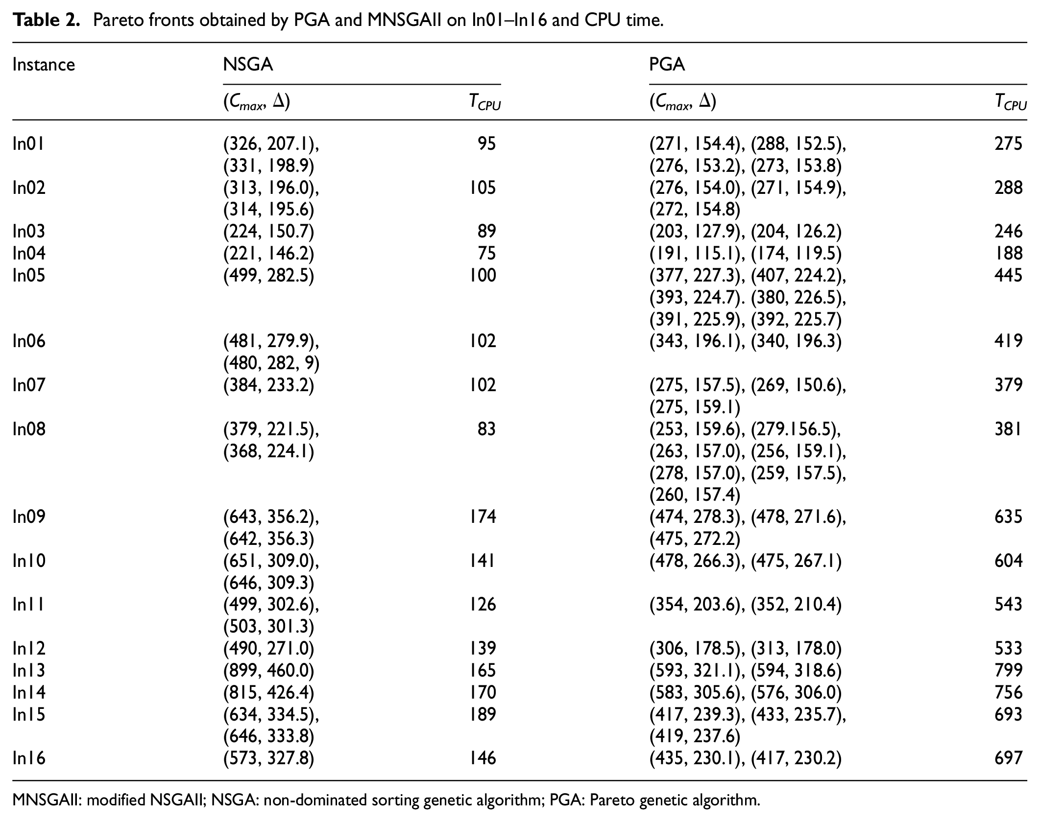
MNSGAII: modified NSGAII; NSGA: non-dominated sorting genetic algorithm; PGA: Pareto genetic algorithm.

Table 3 shows the average value of each index of two algorithms under 10 independent runs of 16 instances. From the table, we can observe that there exist some differences between PGA and MNSGAII on the statistical performance metrics. First, the average number of different non-dominated solutions under MNSGAII is relatively low, for most or many runs, only one Pareto solution is obtained. PGA can obtain more non-dominated solutions than MNSGAII for each instance. This is because MNSGAII does not eliminate individuals with high similarity according to rule (B), although individuals with the same objective values have been eliminated according to rule (A). Note that in the simulation, we found that if the rules (A) and (B) are not used, most individuals in the population would be the same after 200 generations. That is, the population matures very prematurely.

Table 3.

Metric comparison with two objectives.

Instance	Metrics
	N _α		MID		SNS
	NSGAII	PGA	NSGAII	PGA	NSGAII	PGA
In01	1.3	2.6	379.58	306.24	2.13	3.74
In02	1.2	2	367.76	309.12	0.50	2.43
In03	1.2	2.1	285.66	234.95	0.49	1.51
In04	1	2	286.90	214.58	^a	3.25
In05	1.1	2.8	559.61	433.15	2.90	3.30
In06	1.1	1.8	553.17	419.04	0.48	4.08
In07	1.1	2.3	444.43	317.06	5.73	1.11
In08	1	2.8	398.79	295.07	^a	3.45
In09	1.5	1.9	734.15	547.83	3.25	5.56
In10	1.2	2.7	711.88	530.47	3.68	2.60
In11	1.2	2.0	569.52	395.61	1.40	2.02
In12	1.1	2.8	509.64	381.73	0.96	4.23
In13	1.5	2.0	906.96	672.02	0.97	2.11
In14	1.1	1.7	888.14	662.10	0.23	2.68
In15	1.1	2.8	725.05	486.52	7.33	3.97
In16	1	2.7	669.32	458.41	^a	3.45

MID: mean ideal distance; SNS: spread of non-dominated solutions; NSGA: non-dominated sorting genetic algorithm; PGA: Pareto genetic algorithm.

N _α = 1 and SNS is undefined.

The indicators MID and SNS of PGA are also better than those of MNSGAII. This is mainly because the new elitist strategy of PGA is superior to that of MNSGAII and the local search is performed. Hence, it is concluded that PGA is more efficient than MNSGAII for solving our bi-objective scheduling problems.

2. Three-objective optimization: for AMS scheduling problem with three objectives, that is, C_max, Δ, and ϖ, Table 4 lists the ^{Pareto-optimal front}s obtained from a run of PGA and MNSGAII on each instance, and CPU time, and Table 5 shows the average solution number and the average value of MID under 10 independent runs. We can draw similar conclusions as those for AMS scheduling problems with two objectives. From Table 4, we can know that for most simulation instances, PGA can obtain more non-dominated solutions. The only exception is in In14. For this instance, PGA obtains only three solutions, while MNSGAII gets five solutions. But note that each solution obtained by PGA dominates all solutions of MNSGAII. In Table 5, the average value of MID of PGA is less that of MNSGAII. That means that, on average, the solutions obtained by PGA is closer to the optimal solution than that obtained by MNSGAII. For In02, In04, and In07, although MNSGAII obtains more Pareto solutions, the corresponding MID values are much larger than that of PGA, and hence, it can be inferred that PGA has better performance. To sum up, PGA is more effective than MNSGAII for three-objective scheduling problem of deadlock-prone AMSs.

Table 4.

Pareto fronts of three-objective scheduling problem on In01–In16 and CPU time.

Instance	NSGA		PGA
	(C_max, Δ, ϖ)	T_CPU	(C_max, Δ, ϖ)	T_CPU
In01	(311, 182.4, 91.9), (311, 182.0, 92.3),(311, 182.9, 91.4),(311, 181.9, 92.4), (311, 182.5, 91.7)	46	(285, 151.3, 66.4), (271, 153.3, 67.2),(277, 151.8, 67.0), (276, 152.8, 66.9),(275, 152.9, 67.1)	280
In02	(303, 184.9, 91.3), (303, 185.1, 91.2)	38	(263, 156.1, 67.6), (265, 156.1, 66.8),(263, 155.2, 67.7)	221
In03	(246, 154.9, 73.1), (245, 155.9, 74.1)	31	(192, 128.6, 48.3), (191, 130.0, 50.5),(200, 129.0, 48.2), (193, 128.9, 48.3)	174
In04	(230, 144.7, 65.2), (230, 144.8, 65.1)	23	(187, 115.5, 40.5), (196, 115.5, 41.1),(187, 118.2, 40.0), (187, 115.6, 40.4)	214
In05	(564, 299.1, 187.3), (565, 298.9, 187.1)	43	(381, 217.1, 109.9), (373, 219.7, 112.5)	412
In06	(477, 263.9, 154.5), (477, 264.0, 154.3)	59	(371, 202.2, 100.2), (369, 204.3, 102.7)(370, 204.1, 101.8)	419
In07	(391, 220.5, 129.2), (391, 220.7, 129.0)	37	(282, 160.5, 70.7), (271, 161.2, 70.1),(281, 160.7, 69.6), (279, 160.9, 71.1),(278, 161.2, 70.1)	379
In08	(343, 199.8, 107.3), (343, 199.7, 107.4),(343, 199.9, 107.2)	30	(252, 152.3, 63.4), (248, 153.6, 64.8),(254, 153.8, 63.3), (250, 153.0, 64.3),(251, 153.3, 63.8)	339
In09	(650, 349.7, 228.8)	71	(514, 282.4, 167.2), (522, 280.5, 165.0),(517, 281.1, 165.9)	531
In10	(624, 361.3, 243.3), (624, 361.4, 243.3)	48	(498, 269.6, 151.8), (495, 269.6, 152.1),(493, 269.7, 152.0)	514
In11	(462, 251.1, 153.4), (462, 251.0, 153.5),(462, 251.5, 153.0), (462, 251.4, 153.0)	71	(350, 210.6, 113.0), (356, 209.5, 112.0),(355, 209.6, 115.0), (352, 210.0, 112.4)	445
In12	(447, 245.9, 147.2)	55	(307, 177.7, 86.3), (311, 177.6, 86.5)	462
In13	(906, 422.3, 296.3)	92	(610, 336.9, 210.4), (590, 337.8, 211.4),(597, 336.9, 210.4), (591, 337.7, 211.3)	668
In14	(789, 470.4, 342.93), (789, 470.33, 343.0),(789, 470.53, 342.8), (789, 470.47, 342.87)(789, 470.45, 342.88)	57	(578, 308.4, 185.3), (584, 305.8, 182.1),(579, 308.2, 185.3)	690
In15	(646, 344.0, 239.4), (649, 343.8, 239.2)	88	(421, 243.5, 141.7), (428, 240.2, 140.2),(421, 243.3, 143.2), (424, 242.4, 142.5),(425, 242.6, 142.2), (423, 243.2, 142.6)	621
In16	(546, 307.5, 203.7)	98	(399, 218.4, 115.3), (389, 219.8, 116.8),(394, 218.4, 115.3), (391, 218.9, 115.8)	663

NSGA: non-dominated sorting genetic algorithm; PGA: Pareto genetic algorithm.

Table 5.

Metric comparison with three objectives.

Instance	Metrics
	N _α		MID		SNS
	NSGAII	PGA	NSGAII	PGA	NSGAII	PGA
In01	1.8	2.8	380.44	325.30	0.10	2.02
In02	6	4.4	374.14	311.88	0.06	0.78
In03	3.2	6.2	300.40	237.08	0.05	1.89
In04	9.8	5	289.24	222.75	0.09	3.25
In05	2	2.6	577.61	427.22	0.64	3.46
In06	1.2	2.2	570.61	434.23	0.02	1.78
In07	4.2	3.4	449.32	324.82	0.04	2.58
In08	2	4	418.10	310.76	0.02	4.23
In09	1.2	1.6	743.78	573.16	0.03	5.72
In10	1.4	1.8	785.77	545.34	0.04	3.01
In11	1.6	3.2	590.01	418.46	0.04	2.57
In12	1.2	2.2	549.14	386.72	1.07	3.21
In13	1	3.4	964.86	701.48	^a	2.94
In14	2	2.4	938.18	697.98	0.81	3.11
In15	1.2	3	729.13	516.77	1.64	3.60
In16	1	2.6	707.07	476.54	^a	2.70

MID: mean ideal distance; SNS: spread of non-dominated solutions; NSGA: non-dominated sorting genetic algorithm; PGA: Pareto genetic algorithm.

N _α = 1, and SNS is undefined.

Conclusion

This article proposes a PGA for solving the multi-objective scheduling problem of deadlock-prone AMSs with limited resource capacity. A candidate schedule, that is, a sequence of transitions in PN model of AMS, is represented as an individual consisting of route selection and operation sequence. To handle the fitness assignment and solution update in the sense of multi-objective optimization, Pareto dominance and crowding distance in NSGAII are adopted. By introducing new elitist strategy and local search, premature convergence of the population is improved. The feasibility of individuals can be checked based on the PN model of AMS and its deadlock controller, and infeasible individuals can be repaired to feasible ones. Consequently, deadlock is prevented from occurring under the constraint of limited resource capacity, and a deadlock-free schedule is obtained by decoding a feasible individual. Simulation results and comparisons with the MNSGAII in terms of well-known performance metrics show the effectiveness and efficiency of the proposed PGA. The future work is to improve the performance of PGA by considering local search methods and to apply the proposed PGA to solve other AMS scheduling problems with setup and/or uncertain processing time.

Footnotes

Handling Editor: James Baldwin

Declaration of conflicting interests

The author(s) declared no potential conflicts of interest with respect to the research, authorship, and/or publication of this article.

Funding

The author(s) disclosed receipt of the following financial support for the research, authorship, and/or publication of this article: This work was supported, in part, by the National Natural Science Foundation of China under grants 61573269, 61873277, and 71571190 and the Key Research and Development Program of Shaanxi Province under grant 2019GY-056.

References

Pinedo

. Scheduling: theory, algorithms, and systems. 3rd ed. New York: Springer, 2008.

Garey

Johnson

Sethi

. The complexity of flow shop and job shop scheduling. Math Oper Res 1976; 1: 117–129.

Liu

, et al. Robust deadlock control for automated manufacturing systems with unreliable resources based on Petri net reachability graphs. IEEE T Syst Man Cy S 2019; 49: 1371–1385.

Liu

, et al. Elementary siphon-based robust control for automated manufacturing systems with multiple unreliable resources. IEEE Access 2019; 7: 21006–21019.

, et al. Improved multi-step look-ahead control policies for automated manufacturing systems. IEEE Access 2018; 6: 68824–68838.

Liu

Barkaoui

, et al. Robustness of deadlock control for a class of Petri nets with unreliable resources. Inform Sci 2013; 235: 259–279.

Ramaswamy

Joshi

. Deadlock-free schedules for automated manufacturing workstations. IEEE T Robot Autom 1996; 12: 391–400.

Gomes

Barbosa-Povoa

Novais

. Optimal scheduling for flexible job shop operation. Int J Prod Res 2005; 43: 2323–2353.

Toba

. A tight flow control for job-shop fabrication lines with finite buffers. IEEE T Autom Sci Eng 2005; 2: 78–83.

10.

Brucker

Heitmann

Hurink

, et al. Job-shop scheduling with limited capacity buffers. OR Spectrum 2006; 28: 151–176.

11.

Heitmann

. Job-shop scheduling with limited buffer capacities. PhD Thesis, University of Osnabrück, Osnabrück, 2007.

12.

Fahmy

ElMekkawy

Balakrishnan

. Deadlock-free scheduling of flexible job shops with limited capacity buffers. Eur J Ind Eng 2008; 2: 231–252.

13.

Fahmy

ElMekkawy

Balakrishnan

. Mathematical formulations for scheduling in manufacturing cells with limited capacity buffers. Int J Oper Res 2010; 7: 463–486.

14.

Fanti

Zhou

. Deadlock control methods in automated manufacturing systems. IEEE Systs Man Cybern A Systs Humans 2004; 34: 5–22.

15.

Zhou

. Deadlock control of automated manufacturing systems based on Petri nets: a literature review. IEEE T Syst Man Cy C 2012; 42: 437–462.

16.

Giua

. Characterization of admissible marking sets in Petri nets with conflicts and synchronizations. IEEE T Automat Contr 2017; 62: 1329–1341.

17.

Tong

, et al. Basis marking representation of Petri net reachability spaces and its application to the reachability problem. IEEE T Automat Contr 2017; 62: 1078–1093.

18.

Tong

Giua

. On the equivalence of observation structures for Petri net generators. IEEE T Automat Contr 2016; 61: 2448–2462.

19.

Reveliotis

Lawley

Ferreira

. Polynomial-complexity deadlock avoidance policies for sequential resource allocation systems. IEEE T Automat Contr 1997; 42: 1344–1357.

20.

Xing

Zhou

Liu

, et al. Optimal Petri net based polynomial-complexity deadlock avoidance policies for automated manufacturing systems. IEEE T Syst Man Cy A 2009; 39: 188–199.

21.

Ezpeleta

Colom

Martinez

. A Petri net-based deadlock prevention policy for flexible manufacturing system. IEEE T Robot Autom 1995; 11: 173–184.

22.

Zhou

. Deadlock resolution in automated manufacturing systems with robots. IEEE T Autom Sci Eng 2007; 4: 474–480.

23.

Zhou

. Elementary siphons of Petri nets and their application to deadlock prevention in flexible manufacturing systems. IEEE T Syst Man Cy As 2004; 34: 38–51.

24.

Piroddi

Cordone

Fumagalli

. Selective siphon control for deadlock prevention in Petri nets. IEEE T Syst Man Cy A 2008; 38: 1337–1348.

25.

Xing

Han

Zhou

, et al. Deadlock-free genetic scheduling for automated manufacturing systems based on deadlock control policy. IEEE T Syst Man Cy B 2012; 42: 603–615.

26.

Han

Xing

Chen

, et al. Deadlock-free genetic scheduling for flexible manufacturing systems using Petri nets and deadlock controllers. Int J Prod Res 2013; 52: 1557–1572.

27.

Luo

Xing

Zhou

, et al. Deadlock-free scheduling of automated manufacturing systems using Petri nets and hybrid heuristic search. IEEE T Syst Man Cyb 2015; 45: 530–541.

28.

Wang

Xing

, et al. An estimation of distribution algorithm for scheduling problem of flexible manufacturing systems using Petri nets. Appl Math Model 2018; 55: 776–788.

29.

Baruwa

Piera

Guasch

. Deadlock-free scheduling method for flexible manufacturing systems based on timed colored Petri nets and anytime heuristic search. IEEE Trans Syst Man Cybern: Syst 2015; 45: 831–846.

30.

Kacem

Hammadi

Borne

. Approach by localization and multiobjective evolutionary optimization for flexible job-shop scheduling problems. IEEE Syst Man Cybern 2002; 32: 1–13.

31.

Pan

Liang

. An effective hybrid tabu search algorithm for multi-objective flexible job-shop scheduling problems. Comput Ind Eng 2010; 59: 647–662.

32.

Moslehi

Mahnam

. A Pareto approach to multiobjective flexible job-shop scheduling problem using particle swarm optimization and local search. Int J Prod Econ 2011; 129: 14–22.

33.

Rahmati

SHA

Zandieh

Yazdani

. Developing two multiobjective evolutionary algorithms for the multi-objective flexible job shop scheduling problem. Int J Adv Manuf Technol 2013; 64: 915–932.

34.

Shao

Liu

, et al. Hybrid discrete particle swarm optimization for multi-objective flexible job-shop scheduling problem. Int J Adv Manuf Technol 2013; 67: 2885–2901.

35.

Gao

Suganthan

Pan

, et al. Pareto-based grouping discrete harmony search algorithm for multi-objective flexible job shop scheduling. Inform Sciences 2014; 289: 76–90.

36.

Karthikeyan

Asokan

Nickolas

. A hybrid discrete firefly algorithm for multi-objective flexible job shop scheduling problem with limited resource constraints. Int J Adv Manuf Technol 2014; 72: 1567–1579.

37.

Shao

. A Pareto-based estimation of distribution algorithm for solving multiobjective distributed no-wait flow-shop scheduling problem with sequence-dependent setup time. IEEE T Autom Sci Eng 2019; 16: 1344–1360.

38.

Behnamian

Fatemi

Zandieh

. A multi-phase covering Pareto optimal front method to multi-objective scheduling in a realistic hybrid flow shop using a hybrid metaheuristic. Expert Syst Appl 2009; 36: 11057–11069.

39.

Karimi

Zandieh

Karamooz

. Bi-objective group scheduling in hybrid flexible flow shop: a multi-phase approach. Expert Syst Appl 2010; 37: 4024–4032.

40.

Srinivas

Deb

. Multiobjective optimization using nondominated sorting in genetic algorithms. Evol Comput 1994; 2: 221–248.

41.

Deb

. Multi-objective optimization using evolutionary algorithms. New York: John Wiley, 2001.

42.

Deb

Sameer Agarwal

Meyarivan

. A fast and elitist multiobjective genetic algorithm: NSGA-II. IEEE T Evol Comput 2002; 6: 182–197.

A Pareto-based genetic algorithm for multi-objective scheduling of automated manufacturing systems

Abstract

Keywords

Introduction

Modeling of AMSs and deadlock controller based on PNs

PN scheduling models of AMSs

Example 1

Deadlock controllers for PNS

Multi-objective deadlock-free genetic scheduling algorithm for AMSs

Multi-objective optimization problem

Formulation of scheduling problem

Multi-objective scheduling algorithm

Example 2

Algorithm PGA

Simulation results and comparisons

Evaluation metrics

Experimental setup

Results and comparisons

Conclusion

Footnotes

Declaration of conflicting interests

Funding

References