Sage Journals: Discover world-class research

Abstract

This article deals with the numerical study of two-phase shallow flow model describing the mixture of fluid and solid granular particles. The model under investigation consists of coupled mass and momentum equations for solid granular material and fluid particles through non-conservative momentum exchange terms. The non-conservativity of model equations poses major challenges for any numerical scheme, such as well balancing, positivity preservation, accurate approximation of non-conservative terms, and achievement of steady-state conditions. Thus, in order to approximate the present model an accurate, well-balanced, robust, and efficient numerical scheme is required. For this purpose, in this article, Runge–Kutta discontinuous Galerkin method is applied successfully for the first time to solve the model equations. Several test problems are also carried out to check the performance and accuracy of our proposed numerical method. To compare the results, the same model is solved by staggered central Nessyahu–Tadmor scheme. A good comparison is found between two schemes, but the results obtained by Runge–Kutta discontinuous Galerkin scheme are found superior over the central Nessyahu–Tadmor scheme.

Keywords

Two-phase shallow flow model incompressible flow non-conservative hyperbolic system discontinuous Galerkin method central Nessyahu–Tadmor scheme

Introduction

Shallow water flows are characterized by such type of flows in which vertical scale length is considered much smaller than the horizontal scale length. The equations for the shallow flow model can be derived on the basis of basic equations of fluid mechanics by considering incompressible and inviscid fluid. The interaction between the solid granular particles and interstitial fluid appears in the form of rheological behavior of moving mixture of solid grains and fluid. Fluids play a prominent role in the mobility of avalanche flows of solid granular particles. The flow mobility and deformation process are affected by rheological behavior of fluid.¹ Debris flows are example of shallow water flows, and these flows are basically the slurry flows and saturated by water.^2–4 The examples of the debris flows include heavy rainfall, volcanic flows, rock avalanches, mud slides, and landslides.

In this article, two-phase granular flow model describes the flow containing a mixture of granular material and fluid particles. The model contains two mass and two momentum equations which are coupled with each other for both phases.⁴ These equations are connected by non-conservative differential terms.^5–9 Due to the very minute difference between the phase velocities and real eigenstructure, the two-phase shallow flow (TPSF) model is assumed to be hyperbolic, and the model equations are applicable to geophysical flows. In these flows, the inter-phase forces try to move the mixture to maintain kinematic equilibrium. First of all, a Godunov-type finite volume scheme using Roe-type solvers was employed to solve the granular flow models,^6,9 but this method had some disadvantages such as non-preservation of positivity of flow depth and solid volume fraction and unphysical solutions. Hence, this scheme was not suitable for open or free surface flows because it violates the fundamental property of any numerical scheme.⁷ After that, a finite volume scheme based on Riemann solver is applied to address the same model. In the recent literature, some other finite volume schemes have also been applied to investigate the TPSF models. These schemes include central upwind scheme, central Nessyahu–Tadmor (NT) scheme, space–time conservation element and solution element (CESE) scheme, kinetic flux vector splitting (KFVS) scheme, and weighted essentially non-oscillatory (WENO) scheme.^10–14

Discontinuous Galerkin (DG) methods were initially formulated by Cockburn and Shu for non-linear hyperbolic systems. They belong to the class of finite element methods (FEMs) which has several advantages over finite difference methods (FDMs). These methods inherit the geometric flexibility of FEMs and finite volume method (FVMs), retain conservation properties of FVMs, and possess high-order accuracy. DG methods also satisfy the total variation bounded (TVB) property that guarantees the positivity of the scheme.^15–18 In these methods, a simple treatment of B.Cs is adopted to obtain high-order accuracy. In addition, DG methods allow discontinues approximations and produce block-diagonal mass matrices which can be easily converted through algorithms of low computational cost.

In this article, a TVB Runge–Kutta discontinuous Galerkin (RK-DG) method is extended for the first time and applied successfully for solving the TPSF model.^16–18 In the current scheme, DG method deals with space coordinates and converts the given system of coupled partial differential equations (PDEs) into a system of ordinary differential equations (ODEs). The resulting system of ODEs is solved using non-linearly stable and high-order Runge–Kutta method. For validation of the numerical results obtained from the proposed numerical scheme, a staggered central NT scheme is employed to solve the same model equations. A good agreement is found between the results of both schemes, but the results obtained from the RK-DG scheme are dominant over the central scheme results.¹⁹

This article is organized as follows. Section “Incompressible two-phase flow model” is devoted to the introduction of the one-dimensional incompressible two-phase granular flow model. The RK-DG method is presented in section “DG method.” Various numerical case studies are carried out in section “Test problems for TPSF model.” Finally, concluding remarks are given in section “Conclusion.”

Incompressible two-phase flow model

In this section, we consider TPSF model^5–7 which describes the dynamics of shallow thin layer of mixture of the solid granular material and fluid over a smooth horizontal surface. The granular and fluid components of the mixture are assumed to be incompressible with specific densities $ρ_{s}$ and $ρ_{f}$ along with the condition $ρ_{f} < ρ_{s}$ , respectively. Let us consider that $h$ represents the flow height, $ϕ$ denotes the solid volume fraction, and $1 - ϕ$ refers to the volume fraction of fluid. Now we define the solid and fluid heights as

h_{s} = ϕ h and h_{f} = (1 - ϕ) h

(1)

Here, we are considering the one-dimensional flow only, solid and fluid velocities along the x-direction are represented by $u_{s}$ and $u_{f}$ , respectively. Phase momenta of the mixture are given by $m_{s} = h_{s} u_{s}$ and $m_{f} = h_{f} u_{f}$ . The one-dimensional incompressible TPSF model containing the mass and momentum equations for the two constituents can be written as⁷

\partial_{t} h_{s} + \partial_{x} m_{s} = 0

(2)

\begin{matrix} \partial_{t} m_{s} + \partial_{x} (\frac{m_{s}^{2}}{h_{s}} + \frac{g}{2} h_{s}^{2} + \frac{g}{2} (1 - γ) h_{s} h_{f}) + γ g h_{s} \partial_{x} h_{f} \\ = - g h_{s} \partial_{x} b + γ F^{D} \end{matrix}

(3)

\partial_{t} h_{f} + \partial_{x} m_{f} = 0

(4)

\partial_{t} m_{f} + \partial_{x} (\frac{m_{f}^{2}}{h_{f}} + \frac{g}{2} h_{f}^{2}) + g h_{f} \partial_{x} h_{s} = - g h_{f} \partial_{x} b - F^{D}

(5)

Here, g denotes the gravitational constant, $b \overset{def}{=} b (x)$ is the height of the bottom at the point with the coordinate $x$ , and fluid/solid density ratio is given by

γ = \frac{ρ_{f}}{ρ_{s}}

(6)

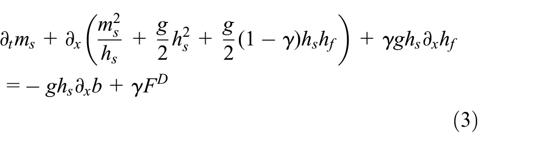
Source terms in term of inter-phase drag force $F^{D}$ are given on the right-hand sides in the momentum equations for both solid and fluid phases. Inter-phase drag force can be expressed as

F^{D} = D (h_{s} + h_{f}) (u_{f} - u_{s})

(7)

where $D = D (ϕ, | u_{f} - u_{s} |; σ)$ is a drag function that generally depends on $| u_{f} - u_{s} |$ and on the set of physical variables $σ$ , for example, specific densities and particle diameter. For $D = 0$ , the above system has similar form as the two-layer shallow flow models.^11,20,21 The main difference between the present model and two-layer shallow flow models is the additional conservative term $\partial_{x} (g ((1 - γ) / 2) h_{s} h_{f})$ in the momentum equation for solid phase of two-phase flow model. In this article, drag forces are neglected. However, the drag effects on the model are important for maintaining flow conditions in the hyperbolic regime. In the compact form, the system can be written as⁷

\frac{\partial w_{k}}{\partial t} + \frac{\partial f_{k}}{\partial x} = τ_{k}, k = 1, 2, 3, 4

(8)

where conserved variables are defined as

\begin{matrix} w_{1} \overset{def}{=} h_{s}, w_{2} \overset{def}{=} m_{s} = h_{s} u_{s}, \\ w_{3} \overset{def}{=} h_{f}, w_{4} \overset{def}{=} m_{f} = h_{f} u_{f} \end{matrix}

(9)

and the fluxes as

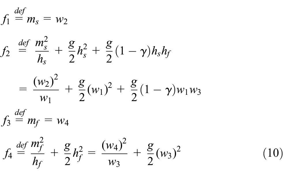
\begin{matrix} f_{1} \overset{def}{=} m_{s} = w_{2} \\ f_{2} \overset{def}{=} \frac{m_{s}^{2}}{h_{s}} + \frac{g}{2} h_{s}^{2} + \frac{g}{2} (1 - γ) h_{s} h_{f} \\ = \frac{{(w_{2})}^{2}}{w_{1}} + \frac{g}{2} (w_{1})^{2} + \frac{g}{2} (1 - γ) w_{1} w_{3} \\ f_{3} \overset{def}{=} m_{f} = w_{4} \\ f_{4} \overset{def}{=} \frac{m_{f}^{2}}{h_{f}} + \frac{g}{2} h_{f}^{2} = \frac{{(w_{4})}^{2}}{w_{3}} + \frac{g}{2} (w_{3})^{2} \end{matrix}

(10)

Moreover, the source terms are expressed as

\begin{matrix} τ_{1} & = 0 = τ_{3}, τ_{2} \overset{def}{=} - γ g h_{s} \frac{\partial h_{f}}{\partial x} - g h_{s} \frac{\partial b}{\partial x} \\ = - γ g w_{1} \frac{\partial w_{3}}{\partial x} - g w_{1} \frac{\partial b}{\partial x} \\ τ_{4} \overset{def}{=} - g h_{f} \frac{\partial h_{s}}{\partial x} - g h_{f} \frac{\partial b}{\partial x} = - g w_{3} \frac{\partial w_{1}}{\partial x} - g w_{3} \frac{\partial b}{\partial x} \end{matrix}

(11)

The conservative and non-conservative fluxes of the system are $f_{k}$ and $τ_{k}$ for $k = 1, 2, 3, 4$ , respectively. Furthermore, the mass equations for $h_{s}$ and $h_{f}$ are conservative; however, the momentum equations for $m_{s}$ and $m_{f}$ account for non-conservative terms of the system related to the dynamics of the solid and fluid phases, respectively. The total momenta of the mixture $m_{m} = m_{s} + γ m_{f}$ can be written as

\partial_{t} m_{m} + \partial_{x} f_{m} (w) = - g (h_{s} + γ h_{f}) \partial_{x} b

(12)

where $w = (w_{1}, w_{2}, w_{3}, w_{4})^{T}$ and $f_{m} (w)$ is defined as

\begin{matrix} f_{m} (w) = f_{2} (w) + γ f_{4} (w) + γ g h_{s} h_{f} \\ = \frac{m_{s}^{2}}{h_{s}} + γ \frac{m_{f}^{2}}{h_{f}} + \frac{g}{2} (h_{s}^{2} + γ h_{f}^{2}) + g \frac{1 + γ}{2} h_{s} h_{f} \end{matrix}

(13)

In the above equation, $f_{2} (w)$ and $f_{4} (w)$ are the second and fourth components of $f_{l} (w)$ defined in equation (10). The quasi-linear form of the above model is

\partial_{t} w + A (w) \partial_{x} (w) = ψ^{b} (w)

(14)

where $ψ^{b} (w) = (0, - g h_{s} \partial_{x} b, 0, - g h_{f} \partial_{x} b)^{T}$ , and the coefficient matrix $A (w)$ is given by

A (w) = (\begin{matrix} 0 & 1 & 0 & 0 \\ g h_{s} - u_{s}^{2} + g (\frac{1 - γ}{2}) h_{f} & 2 u_{s} & g (\frac{1 - γ}{2}) h_{s} & 0 \\ 0 & 0 & 0 & 1 \\ g h_{f} & 0 & g h_{f} - u_{f}^{2} & 2 u_{f} \end{matrix})

(15)

The set of values which are admissible for this model is

Ω = {w \in R^{4}; h_{s}, h_{f} \geq 0 and u_{s}, u_{f} \in R}

(16)

in terms of $h = h_{s} + h_{f}$ and $ϕ = h_{s} / (h_{s} + h_{f})$ , we can write

Ω = {w \in R^{4}; h \geq 0, ϕ \in [0, 1], and u_{s}, u_{f} \in R}

(17)

Steady states for the model

The steady-state conditions for the model (8) are

h_{s} u_{s} = constant, h_{f} u_{f} = constant

(18)

\frac{u_{f}^{2}}{2} + g (h_{s} + h_{f} + b) = constant

(19)

h_{s} \partial_{x} (\frac{u_{f}^{2}}{2} - \frac{u_{s}^{2}}{2} + g \frac{1 - γ}{2} h_{f}) - h_{f} \partial_{x} (g \frac{1 - γ}{2} h_{s}) = 0

(20)

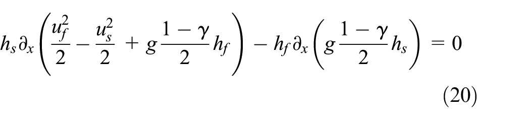
From the above conditions, it simplifies to $(h_{s} + h_{f} + b) = constant,$ and $h_{s} / h_{f} = constant,$ for a special case of steady state $(u_{s} = u_{f} = 0)$ . In the form of physical variables $h = h_{s} + h_{f}$ and $ϕ = h_{s} / h_{s} + h_{f}$ , the equilibrium at rest is characterized by

h + b = constant and ϕ = constant

(21)

Eigenvalues and hyperbolicity of the model

In general, explicit expressions for the eigenvalues of the jacobian matrix of incompressible two-phase shallow granular flow model cannot be found straightforwardly. But, in particular cases, eigenvalues can be calculated from the Jacobian matrix:

Case I: when solid and fluid velocities are taken as equal, that is, $u_{s} = u_{f} = u$ and $(φ \neq 1)$ , then the eigenvalues are real and distinct. In this case, eigenvalues are given as

λ_{1, 4} = u \mp c and λ_{2, 3} = u \mp c μ

where $c = \sqrt{gh}$ and $μ = \sqrt{\frac{(1 - φ) (1 - γ)}{2}}$ . Hence, in this case, our model is hyperbolic.

Case II: when $φ = 0$ , the eigenvalues are

\begin{matrix} λ_{1, 2} = u_{f} \mp c, λ_{3, 4} = u_{s} \mp c μ with \\ c = \sqrt{gh} and μ = \sqrt{\frac{1 - γ}{2}} \end{matrix}

Case III: when $φ = 1$ , in this case, we can find two distinct eigenvalues $λ_{1, 2} = u_{s} \mp c$ and double eigenvalue $λ_{3, 4} = u_{f} .$

DG method

In this section, the one-dimensional incompressible two-phase flow model is considered. In one space dimension, two-phase model in equation (8) reduces to

\frac{\partial w}{\partial t} + \frac{\partial f (w)}{\partial x} = T (w)

(22)

where

w = (h_{s}, m_{s}, h_{f}, m_{f})^{T}

(23)

f (w) = {(m_{s}, \frac{m_{s}^{2}}{h_{s}} + \frac{g}{2} h_{s}^{2} + \frac{g}{2} (1 - γ) h_{s} h_{f}, m_{f}, \frac{m_{f}^{2}}{h_{f}} + \frac{g}{2} h_{f}^{2})}^{T}

(24)

T (w) = {(0, γ g h_{s} \frac{\partial h_{f}}{\partial x} - g h_{s} \frac{\partial b}{\partial x}, 0, - g h_{f} \frac{\partial h_{s}}{\partial x} - g h_{f} \frac{\partial b}{\partial x})}^{T}

(25)

Here, $w$ , $f$ , and $T$ are the vectors of conservative variables, fluxes, and source terms, respectively. Moreover, $h_{s} = h ϕ$ , $h_{f} = h (1 - ϕ)$ , $m_{s} = h_{s} u_{s}$ , and $m_{f} = h_{f} u_{f}$ are the solid height, fluid height, solid momentum, and fluid momentum, respectively. Furthermore, total height is $h = h_{s} + h_{f} .$

For the numerical treatment of the model (8), a TVB RK-DG scheme^16,17 is implemented for the discretization of space coordinate only. The derivatives of time coordinate are discretized using TVB Runge–Kutta method.

In order to discretize the spatial domain $[x_{0}, x_{max}]$ , we proceed as follows. For $j = 0, 1, 2, \dots, N$ , let $x_{j + (1 / 2)}$ be the cells partitions, $I_{j} = (x_{j - (1 / 2)}, x_{j + (1 / 2)})$ be the domain of cell $j$ , $Δ x_{j} = x_{j + (1 / 2)} - x_{j - (1 / 2)}$ be the width of cell $j$ , and $I = U I_{j}$ be the union of partitions in the whole domain. We seek an approximate solution $w_{h} (t, x)$ to $w (t, x)$ such that for each time $t \in 0, t_{max}],$ $w_{h} (t, x)$ belongs to the finite dimensional space

V_{h} = {v \in h^{1} (I) : v |_{I_{j}} \in P^{k} (I_{j}), j = 0, 1, 2, \dots, N}

(26)

where $P^{k} (I_{j})$ represents the space of polynomials in $I_{j}$ of degree at most $k$ . Note that in $V_{h}$ , the functions are allowed to have jumps at the cell interface $x_{j + (1 / 2)}$ . To determine the approximate solution $w_{h} (t, x)$ , a weak formulation is needed, which is usually obtained by multiplying equation (22) with a smooth function $v (x)$ and by integrating over the interval $I_{j}$ . After using integration by parts, the weak formulation appears in the following form

\begin{matrix} \int_{I_{j}} \frac{\partial w (t, x)}{\partial t} v (x) dx = \int_{I_{j}} f (w (t, x)) \frac{\partial}{\partial x} v (x) dx + \int_{I_{j}} τ (w (t, x)) v (x) dx \\ - [f (w (t, x_{j + \frac{1}{2}})) v (x_{j + \frac{1}{2}}) - f (w (t, x_{j - \frac{1}{2}})) v (x_{j - \frac{1}{2}})] \end{matrix}

(27)

One way to apply equation (26) is to choose Legendre polynomials, $P_{l} (x)$ , of order $l$ as local basis functions. In this approach, the L²-orthogonality property of Legendre polynomials can be exploited, written as

\int_{- 1}^{1} P_{l} (s) P_{l'} (s) ds = (\frac{2}{2 l + 1}) δ_{ll'}

(28)

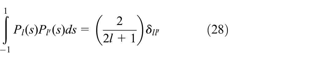
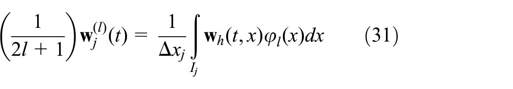
For each $x \in I_{j}$ , the solution $w_{h}$ can be expressed as

w_{h} (t, x) = \sum_{l = 0}^{k} w_{j}^{(l)} φ_{l} (x)

(29)

where

φ_{l} (x) = P_{l} (2 (x - x_{j}) / Δ x_{j})

(30)

It can be easily proved that

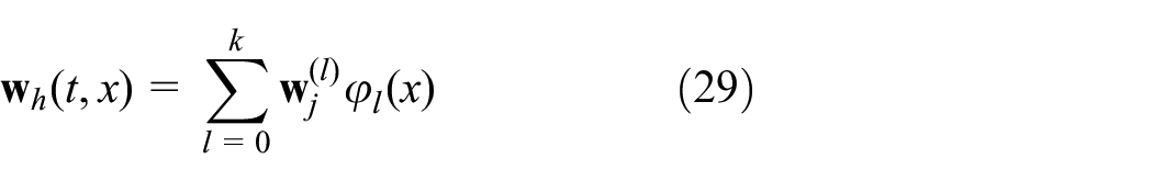
(\frac{1}{2 l + 1}) w_{j}^{(l)} (t) = \frac{1}{Δ x_{j}} \int_{I_{j}} w_{h} (t, x) φ_{l} (x) dx

(31)

Since the above Legendre polynomials are used as local basis functions, the smooth function $v (x)$ can be replaced by the test function $φ_{l} \in V_{h}$ and the exact solution $w$ by the approximate solution $w_{h}$ . Moreover, the function $w_{j + (1 / 2)} = w (t, x_{j + (1 / 2)})$ is not known at the cell interface $x_{j + (1 / 2)}$ . Therefore, the flux $f (w (t, x))$ has to be approximated by a numerical flux that depends on two values of $w_{h} (t, x)$ , that is

f (w (t, x_{j + \frac{1}{2}})) \approx h_{j + \frac{1}{2}} = h (w (t, x_{j + \frac{1}{2}}^{-}), w (t, x_{j - \frac{1}{2}}^{+}))

(32)

Here

w_{j + \frac{1}{2}}^{-} = w_{h} (t, x_{j + \frac{1}{2}}^{-}) = \sum_{l = 0}^{k} w_{j}^{(l)} φ_{l} (x_{j + \frac{1}{2}})

(33)

w_{j - \frac{1}{2}}^{+} = w_{h} (t, x_{j - \frac{1}{2}}^{+}) = \sum_{l = 0}^{k} w_{j}^{(l)} φ_{l} (x_{j - \frac{1}{2}})

(34)

Using the above definitions, the weak formulation in equation (27) simplifies to

\begin{matrix} \frac{d w_{j}^{(l)} (t)}{dt} = - \frac{2 l + 1}{Δ x_{j}} \\ (h_{j + \frac{1}{2}} φ_{l} (x_{j + \frac{1}{2}}) - h_{j - \frac{1}{2}} φ_{l} (x_{j - \frac{1}{2}})) \\ + \frac{2 l + 1}{Δ x_{j}} \int_{I_{j}} (f (w_{h} (t, x)) \frac{d φ_{l} (x)}{dx}) dx \\ + \frac{2 l + 1}{Δ x_{j}} \int_{I_{j}} (τ (w_{h} (t, x)) φ_{l} (x) dx \end{matrix}

(35)

It remains to choose the appropriate numerical flux function $h$ . The above equations define a monotone scheme if the numerical flux function $h (a, b)$ is consistent, $h (w, w) = f (w)$ , and satisfies the Lipschitz continuity condition, that is, $h (a, b)$ is a non-decreasing function of its first argument and non-increasing function of its second argument.^22,23 The two following numerical flux functions are used that satisfy the above properties:^22–24

1. The Lax–Friedrichs flux

h^{LF} (a, b) = \frac{1}{2} [f (a) + f (b) - C (b - a)]

(36)

C = max_{inf w^{(0)} (x) \leq s \leq sup w^{(0)} (x)} | f' (s) |

(37)

2. The Local Lax–Friedrichs flux

h^{LLF} (a, b) = \frac{1}{2} [f (a) + f (b) - C (b - a)]

(38)

C = max_{min (a, b) \leq s \leq max (a, b)} | f' (s) |

(39)

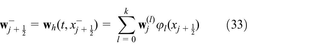
The Gauss–Lobatto quadrature formula of 10th order was used to approximate numerically integral terms coming on the right-hand side of equation (35). To achieve local maximum principle with respect to the means, some limiting procedure is needed. For that purpose, it is required to modify the interface values $w_{j \pm (1 / 2)}^{\pm}$ in equations (32)–(34) by some local projection limiter. At this end, equations (33) and (34) can be written as^16,17

w_{j + \frac{1}{2}}^{-} = w_{j}^{(0)} + {\tilde{w}}_{j}, w_{j - \frac{1}{2}}^{+} = w_{j}^{(0)} - {\hat{w}}_{j}

(40)

where

{\tilde{w}}_{j} = \sum_{l = 1}^{k} w_{j}^{(l)} φ_{l} (x_{j + \frac{1}{2}}), {\hat{w}}_{j} = - \sum_{l = 1}^{k} w_{j}^{(l)} φ_{l} (x_{j - \frac{1}{2}})

(41)

Next, ${\tilde{w}}_{j}$ and ${\hat{w}}_{j}$ can be modified as

{\tilde{w}}_{j}^{(\mod)} = mm ({\tilde{w}}_{j}, Δ_{+} w_{j}^{(0)}, Δ_{-} w_{j}^{(0)})

(42)

{\hat{w}}_{j}^{(\mod)} = mm ({\hat{w}}_{j}, Δ_{+} w_{j}^{(0)}, Δ_{-} w_{j}^{(0)})

(43)

where $Δ_{\pm} w_{j} = \pm (w_{j \pm 1} - w_{j})$ and mm is the usual minmod function which is defined as

\begin{matrix} mm (a_{1}, a_{2}, a_{3}) = \\ {\begin{matrix} s \cdot min_{1 \leq j \leq 3} | a_{i} | & if sign (a_{1}) = sign (a_{2}) = sign (a_{3}) = s \\ 0 & otherwise \end{matrix} \end{matrix}

(44)

Then, equation (40) modifies to

w_{j + \frac{1}{2}}^{- (\mod)} = w_{j}^{(0)} + {\tilde{w}}_{j}^{(\mod)}, w_{j - \frac{1}{2}}^{+ (\mod)} = w_{j}^{(0)} - {\hat{w}}_{j}^{(\mod)}

(45)

and equation (32) is replaced by

h_{j + \frac{1}{2}} = h (w_{j + \frac{1}{2}}^{- (\mod)}, w_{j - \frac{1}{2}}^{+ (\mod)})

(46)

This limiter corresponds to adding the minimum amount of numerical diffusion while preserving the stability of the scheme. The DG method in addition to the above-explained slope limiter has proved to be stable.²⁵

But, in this scheme, we used the WENO limiter²⁶ to eliminate oscillations and enforce the stability. In this way, first identify “troubled cells,” namely, those cells that need to be reconstructed. A troubled cell is defined as if one of the minmod functions given in equations (42) and (43) gets active (returns other than the first argument) and is marked for further reconstructions. For the troubled cells, we would like to reconstruct the polynomial solution while retaining its cell average.

Finally, a Runge–Kutta method is implemented that maintains the TVB property needed to solve the resulting system of ODE. Let us rewrite equation (35) in a concise form as

\frac{d w_{h}}{dt} = L_{h} (t, w_{h})

(47)

Then, the r-order TVB Runge–Kutta method can be used to approximate equation (47)

\begin{matrix} w_{h}^{(k)} = \sum_{l = 0}^{k - 1} [α_{kl} w_{h}^{(l)} + β_{kl} Δ t L_{h} (t^{n} + d_{l} Δ t, w_{h}^{(l)})], \\ k = 1, 2, \dots, r \end{matrix}

(48)

were based on the boundary conditions

w_{h}^{(0)} = w_{h}^{n}, w_{h}^{(r)} = w_{h}^{n + 1}

(49)

For the second-order TVB Runge–Kutta method, the coefficient are given as^15,16

\begin{matrix} α_{10} = β_{10} = 1, α_{20} = α_{21} = β_{21} = \frac{1}{2}, \\ β_{20} = 0; d_{0} = 0, d_{1} = 1 \end{matrix}

(50)

While, for the third-order TVB Runge–Kutta method, the coefficient are given as

\begin{matrix} α_{10} = β_{10} = 1, α_{20} = \frac{3}{4}, β_{20} = 0, \\ α_{21} = β_{21} = \frac{1}{4}, α_{30} = \frac{1}{3} \\ β_{30} = α_{31} = β_{31} = 0, α_{32} = β_{32} = \frac{2}{3}, \\ d_{0} = 0, d_{1} = 1, d_{2} = \frac{1}{2} \end{matrix}

(51)

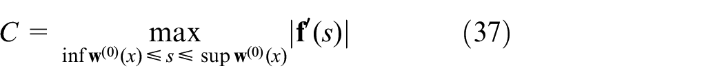
In order to guarantee numerical convergence and stability of the DG scheme, the time step is taken according to the following Courant–Friedrichs–Lewy (CFL) condition^16,23

Δ t \leq (\frac{1}{2 k + 1}) \frac{min (Δ x_{j})}{λ_{\max}}

(52)

where $λ_{\max}$ is the maximum eigenvalue of the Jacobian matrix $\partial f (w) / \partial w$ , and $k = 1, 2$ for the second- and third-order schemes, respectively. This time step is adaptive, which reduces for the case of large variations (large slopes) in the solution and increases otherwise.

Test problems for TPSF model

In this section, we present some numerical case studies to analyze the performance of our proposed RK-DG method for the proposed model. In all the test problems, we set $γ = 0.5$ . The numerical results of RK-DG method¹⁶ are compared with those obtained from the central NT scheme.¹⁹

Problem 1: simple Riemann problem

This Riemann problem was considered in Qamar et al.⁵ and Pelanti et al.⁶ The left and right states of the initial data are given as

(h, ϕ, u_{s}, u_{f})_{L} = (1.0, 0.8, 0.0, 0.0), if x \leq 0.0

(53)

(h, ϕ, u_{s}, u_{f})_{R} = (2.0, 0.4, - 0.9, - 0.1), if x > 0.0

(54)

The computational domain $[- 5, 5]$ is divided into $200$ grid points and the bottom is flat, that is, $b (x) = constant$ . Reference solution is calculated from RK-DG method on $800$ grid points. The simulation results for total height $h$ , solid height $h_{s}$ , fluid height $h_{f}$ , solid volume fraction $ϕ$ , and the velocities $u_{s}$ and $u_{f}$ computed at $200$ grid points from RK-DG and central schemes at $t = 0.5$ , which are displayed in Figure 1. The L¹-errors are computed for flow height and solid volume fraction with respect to reference solution and are displayed in Table 1. The L¹-errors in both schemes are functions of grid points which are shown in Figure 2. It can be observed that RK-DG method produces less errors as compared to central NT scheme in the solutions. The numerical solution consists of a 1-rarefaction wave, a 2-shock wave, a 3-rarefaction wave, and a 4-shock wave. The results of RK-DG method are compared with the reference solution and solution obtained from staggered central NT schemes. It can be observed that both schemes give comparable results. Moreover, results given by our proposed method show good agreement with those presented in Qamar et al.⁵ and Pelanti et al.⁶

Figure 1.

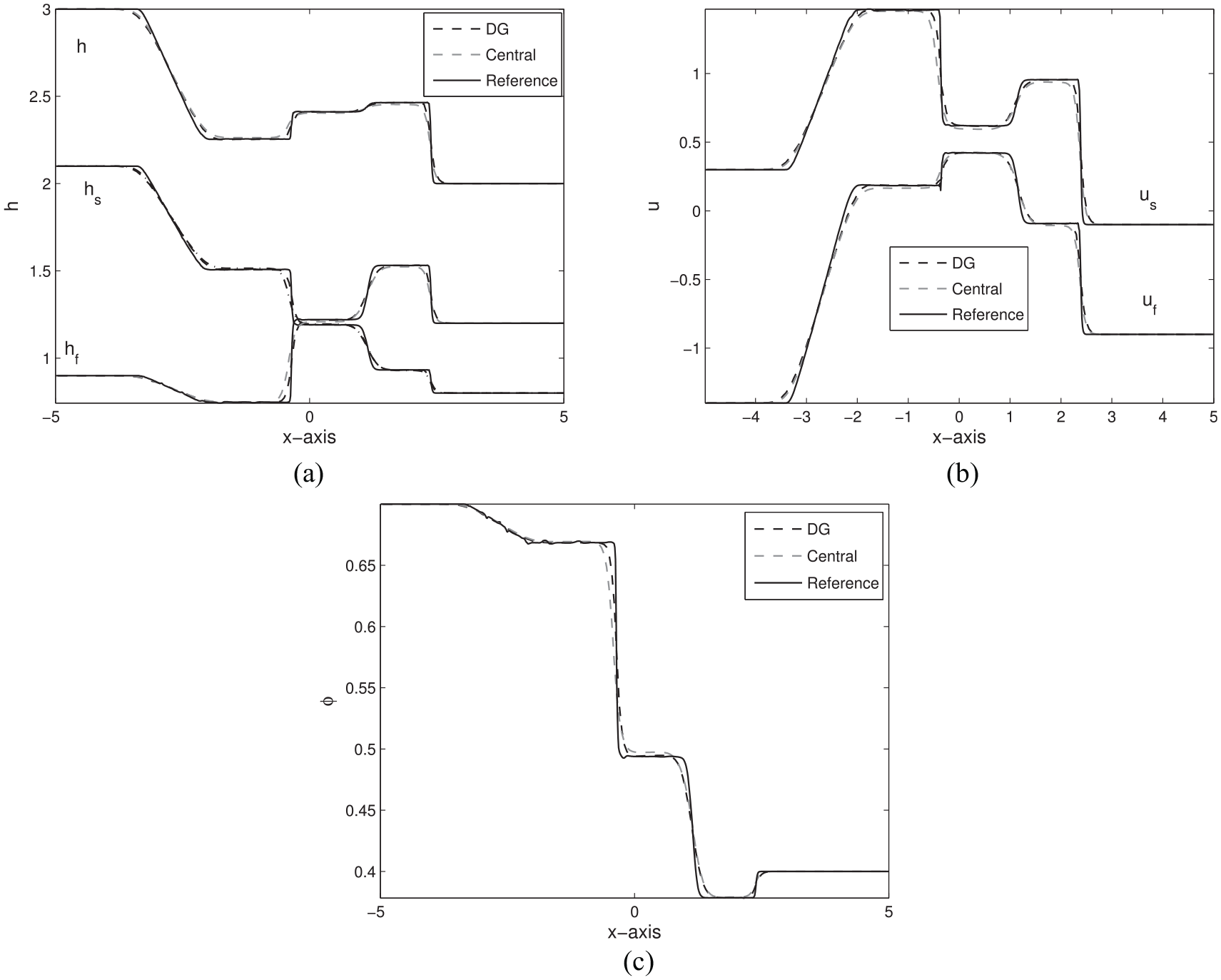
Problem 1: simple Riemann problem. Comparison of DG and central NT schemes at time $t = 0.5$ .

Table 1.

Problem 1: comparison of L¹-errors.

N	Height (h)		Solid volume fraction $(ϕ)$		Solid velocity $(u_{s})$		Fluid velocity $(u_{f})$
	DG	Central	DG	Central	DG	Central	DG	Central
50	0.331	0.331	0.095	0.095	0.719	0.719	0.840	0.840
100	0.164	0.176	0.041	0.051	0.377	0.387	0.399	0.462
200	0.084	0.085	0.024	0.026	0.188	0.189	0.209	0.222
400	0.029	0.034	0.009	0.012	0.069	0.072	0.079	0.089
800	0.008	0.009	0.002	0.002	0.017	0.021	0.019	0.022

DG: discontinuous Galerkin.

Figure 2.

Problem 1: convergence study of DG and central NT schemes. Comparison of L¹-errors in height, solid volume fraction, solid velocity, and fluid velocity in both schemes at different grid points.

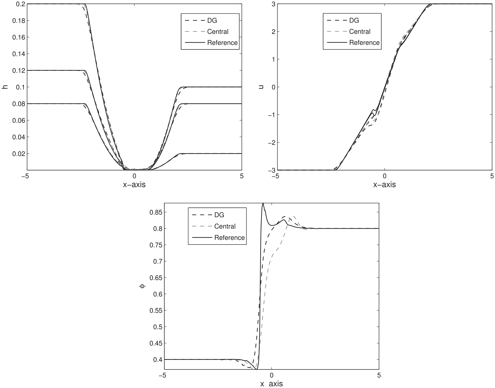
Problem 2: rarefaction of the fluid constituent into vacuum

This problem was also considered in Qamar et al.⁵ and Pelanti et al.⁶ Here, we consider the flow for $h > 0$ , $x \in R$ , and $t > 0$ . The fluid mixture height is same over the whole domain $[- 5, 5]$ . The state on the right-hand side for the fluid phase is nearly vacuum zone. The initial data for Riemann problem in both states are

(h, ϕ, u_{s}, u_{f})_{L} = (1.0, 0.8, 0.0, 0.0), if x \leq 0.0

(55)

(h, ϕ, u_{s}, u_{f})_{R} = (1.0, 1.0, 0.0, 0.0), if x > 0.0

(56)

The bottom is flat, that is, $b (x) = constant$ , the discontinuity is located at $x = 0.0$ , and the gravity constant is $g = 9.81$ . The whole computational domain $[- 5, 5]$ is divided into $200$ mesh cells. Numerical results are obtained from both RK-DG method and central NT scheme with $200$ grid points at $t = 1.0$ , and $800$ mesh cells are used for the reference solution obtained from RK-DG method. For the numerical simulations, we considered $ϕ = 1 - 10^{- 6}$ on the right-hand side to avoid division by zero and the inconvenience in the algorithm. Another purpose to take this value is to recover the conservative variables. The numerical results are shown in Figure 3. The Riemann solution for the mixture contains 2-rarefaction waves across which $h_{f} = h (1 - ϕ)$ vanishes. Moreover, in the left zone which is purely solid phase, a 1-shock wave and a 4-rarefaction wave occurs. Finally, the numerical results of both schemes are compared, it was found that RK-DG method gives superior results than central NT scheme, and its results are in good agreement with those presented in Qamar et al.⁵ and Pelanti et al.⁶

Figure 3.

Problem 2: rarefaction of the fluid constituents into vacuum (Dam break problem). Comparison of DG and central NT schemes at time $t = 1$ .

Problem 3: spreading of a granular mass

This numerical experiment was also taken from Qamar et al.⁵ and Pelanti et al.⁶ In this experiment, the granular mass is spread over a horizontal surface. Initially, $u_{s} = u_{f} = 0$ and flow height in addition with solid volume fraction are taken as

h (x) = {\begin{matrix} 1.0, & - 1 \leq x \leq 1 \\ 0.0, & otherwise \end{matrix} and ϕ (x) = \frac{1}{10} (4 e^{- x^{2}} + 3) at t = 0

(57)

In this case, the bottom is flat, that is, $b (x) = constant$ , $g = 1$ , and flow height $h$ is taken as zero below the tolerance $\in = 10^{- 5}$ . The computational domain [–10, 10] is subdivided into $200$ grid points. In the absence of drag forces, the difference between the phase velocities, that is, $| u_{s} - u_{f} | \to 0$ as $h \to 0$ . The computational results by RK-DG method and central NT scheme are obtained at $200$ mesh cells and are depicted in the Figure 4. The reference solution is obtained by RK-DG method at $800$ mesh cells. There is a prominent change in the behavior of solid volume fraction, and clearly the hyperbolic conditions are maintained as total height of flow vanishes. The numerical results of RK-DG and central NT schemes are in closer agreement with each other and with the reference solution. However, RK-DG method has superior results.

Figure 4.

Problem 3: spreading of granular mass with no drag forces. Comparison of DG and central NT schemes at time $t = 4.0$ .

Problem 4: dry bed generation

This problem is concerned with the generation of dry bed zone. In this problem, three further cases of the Riemann problem are discussed. In all the three cases, the solutions consist of two opposite moving rarefaction waves, and a dry bed region is generated. The initial data for the three test problems are given in Table 2.

Table 2.

Problem 4: initial data for test cases of dry bed formation.

$No .$	$(ϕ, h, u_{s}, u_{f})_{L}$	$(ϕ, h, u_{s}, u_{f})_{R}$
$1$	$(0.1, 0.4, - 3.0, - 3.0)_{L}$	$(0.1, 0.7, 3.0, 3.0)_{R}$
$2$	$(0.4, 0.4, 0.0, 0.0)_{L}$	$(0.1, 0.7, 6.0, 6.0)_{R}$
$3$	$(0.2, 0.4, - 3.0, - 3.0)_{L}$	$(0.1, 0.8, 3.0, 3.0)_{R}$

In all the three test problems, initially the interface is located at $x = 0$ . The gravity constant is taken as $g = 9.81$ and the bottom is considered as flat, that is, $b (x) = constant$ , the computational domain $- 5 \leq x \leq 5$ is divided into $200$ mesh cells for numerical solution and $800$ cells for reference solution.

In our model, no inter-phase drag forces are considered. As both fluids are separate at $x = 0$ , a vacuum region is generated, and this vacuum region is captured in the plots of height in Figures 5 –7. This region is clearly indicated in Figures 5 and 7 as compared to Figure 6. Test case $1$ is most similar to the test problem $1$ . The computational results calculated at $t = 1$ for flow height $h$ , the solid phase height and fluid phase height $h_{s}$ and $h_{f}$ , momenta of both phases $m_{s}$ and $m_{f}$ , momentum of mixture $m_{m} = m_{s} + m_{f}$ , the SVP $ϕ$ , and velocities $u_{s} and u_{f}$ , respectively, are depicted in Figure 5. The numerical results of RK-DG method and central NT scheme at $200$ grid points are compared with each other and with the reference results obtained by RK-DG method at $800$ grid points. However, from the comparison, it was observed that RK-DG method gives high resolution of the discontinuous profiles.

Figure 5.

Problem 4a: dry bed generation. Comparison of DG and central NT schemes at time $t = 1$ .

Figure 6.

Problem 4b: dry bed generation. Comparison of DG and central NT schemes at time $t = 0.5$ .

Figure 7.

Problem 4c: dry bed generation. Comparison of DG and central NT schemes at time $t = 0.5$ .

Test case $2$ is analogous to test case $1$ and problem $1$ . The only difference is that here we take translation in velocities so that left transonic rarefaction is visible. The numerical results from both schemes are displayed in Figure 6. Again, a better performance of RK-DG method can be observed.

In test case $3$ , the flow height and solid volume fraction contain the initial discontinuity. Finally, the numerical results are displayed in Figure 7, and it can be seen clearly that the both schemes have comparable results.

Problem 5: interface propagation

This problem is considered to verify the performance of our proposed RK-DG method to capture and propagate the discontinuities over time. In order to validate the schemes, this example has been widely used for multi-layer flows.^27,28 The initial data for this problem are given by

(h_{s}, h_{f}, u_{s}, u_{f})_{L} = (0.5, 0.5, 2.5, 2.5), if x \leq 0.5

(58)

(h_{s}, h_{f}, u_{s}, u_{f})_{R} = (0.55, 0.45, 2.5, 2.5), if x > 0.5

(59)

Initially, the location of interface is at $x = 0.5$ . The bottom is taken as flat, that is, $b (x) = constant$ ; the value of acceleration due to gravity constant is taken as $g = 9.812$ ; and for this problem, $γ = ρ_{s} / ρ_{f} = 0.5$ . The domain is $[0, 1]$ is discretized into $200$ mesh cells for the numerical solution from RK-DG and central NT schemes, and $800$ cells are used for the reference solution of RK-DG method. The results are displayed in Figure 8 show the evolution of interface between two layers, free surface displacement, and the velocity of each layer. It can be observed that the results obtained from the both schemes are comparable. However, RK-DG method has the good ability to resolve shock discontinuities.

Figure 8.

Problem 5: interface propagation. Comparison of DG and central NT schemes at time $t = 0.1$ .

Problem 6: perturbation of a steady state at rest

In order to confirm the well-balanced property of the proposed RK-DG method, we consider a test problem incorporating non-flat bottom topography. The same test problem was presented in Qamar et al.⁵ and Pelanti et al.⁶ In this way, we added a discontinuous rectangular topography in the right-hand side of the model to check the ability of our suggested well-balanced scheme. In this problem, we study the behavior of a small perturbation which satisfies the steady-state conditions at rest given in equation (18) over a variable bottom topography defined as

b (x) = {\begin{matrix} 0.25 (\cos (10 π (x - 1 / 2)) + 1), & if | x - 0.5 | < 0.1 \\ 0 & otherwise \end{matrix}

(60)

Initially, we take a small perturbation of the flow depth $h$ and of the solid volume fraction $ϕ$

\begin{matrix} h (x, 0) = h_{o} + \tilde{h}, ϕ (x, 0) = ϕ_{o} - \tilde{ϕ}, for \\ - 0.6 < x < - 0.5 \end{matrix}

(61)

where $h_{o} = 1$ , $ϕ_{o} = 0.6$ , and $\tilde{h} = \tilde{ϕ} = 10^{- 3}$ . The domain of the problem is $[- 0.9, 1.1]$ , which is discretized into $200$ grid points for numerical solution and $800$ mesh points for reference solution at four different times. The values of constants are taken as $g = 1$ and $γ = 1 / 2$ . Moreover, free flowing boundary conditions are used. The L¹-errors are computed for flow height and solid volume fraction with respect to reference solution and are displayed in Table 3. The L¹-errors in both schemes are functions of grid points which are shown in Figure 9.

Table 3.

Problem 6: comparison of L¹-errors in the schemes.

N	Total height $(h + b)$		Solid volume fraction $(ϕ)$
	DG	Central	DG	Central
50	1.76 × 10⁻⁵	2.31 × 10⁻⁵	5.21 × 10⁻⁵	7.24 × 10⁻⁵
100	1.36 × 10⁻⁵	1.48 × 10⁻⁵	3.79 × 10⁻⁵	5.27 × 10⁻⁵
200	1.06 × 10⁻⁵	1.15 × 10⁻⁵	2.26 × 10⁻⁵	3.45 × 10⁻⁵
400	8.65 × 10⁻⁶	9.55 × 10⁻⁶	1.13 × 10⁻⁵	1.54 × 10⁻⁵
800	4.27 × 10⁻⁶	5.25 × 10⁻⁶	6.56 × 10⁻⁶	1.07 × 10⁻⁵

DG: discontinuous Galerkin.

Figure 9.

Problem 6: convergence study of DG and Central NT schemes. Comparison of L¹-errors in total height and solid volume fraction in both schemes at different grid points.

It is very clear from the set of first three figures displayed in Figure 10 that the initial perturbation splits into four waves, two left-going waves, and two right-going waves that leave the domain from the left edge, Figure 10 shows at $t = 1.5$ that the right-going external wave has just passed over the obstacle at the bottom, and it has been partially reflected. After reflection, this right-going wave has escaped out from the right boundary of the domain and the reflected wave generated by right-going wave has passed through the incoming right wave. The last part shown in Figure 10 represents the final situation in which all the disturbances have exited from the computational region and finally steady-state equilibrium is attained at $t = 6.25$ . Finally, we compared the results of RK-DG method with the reference solution and staggered central NT scheme¹⁹ at different times $t = 0.25$ , $t = 0.25$ , $t = 2$ , $t = 4$ , and $t = 6.25$ in Figure 10. It can be concluded that the results of central NT scheme gives more diffusive solution compared to the RK-DG method.

Figure 10.

Problem 6: perturbation of a steady state at rest. Comparison of DG and central NT schemes at time $t = 0.25$ , $t = 1.5$ , $t = 2.0$ , $t = 4.0$ , and $t = 6.25$ .

Those numerical schemes which are not well-balanced present in the literature may produce unphysical disturbances in such kind of numerical test cases.²⁹ Hence, our computational methods have the ability to capture physically correct reflected waves, without producing spurious oscillations in the simulated results.

Conclusion

In this article, a high-resolution RK-DG method was extended for the first time to address the incompressible TPSF model. Our proposed numerical scheme has the good ability to capture sharp discontinuities and avoids spurious oscillations in the solutions. The performance and accuracy of the proposed scheme were checked quantitatively and qualitatively by considering several numerical case studies. It was observed that the present scheme effectively captures all the sharp discontinuities in the solutions, and preserves the positivity of the flow variables like flow height and volume fraction. For validation and comparison, the central NT scheme was also applied to the same model equations. A good agreement was found between the results of both schemes. However, it was observed that the RK-DG scheme gives better resolution of the sharp discontinuities produced in the profiles of physical parameters.

Footnotes

Handling Editor: James Baldwin

Declaration of conflicting interests

The author(s) declared no potential conflicts of interest with respect to the research, authorship, and/or publication of this article.

Funding

The author(s) received no financial support for the research, authorship, and/or publication of this article.

ORCID iD

Muhammad Rehan Saleem

References

Legros

. The mobility of long-runout landslides. Eng Geol 2002; 63: 301–331.

Iverson

Denlinger

. Flow of variably fluidized granular masses across three-dimensional terrain 1. Coulomb mixture theory. J Geophys Res 2001; 106: 537–552.

Major

Iverson

. Debris-flow deposition, effects of pore-fluid pressure and friction concentrated at flow margins. GSA Bull 1999; 111: 1424–1434.

Pitman

. A two-fluid model for avalanche and debris flows. Philos Trans Roy Soc A 2005; 363: 1573–1601.

Qamar

Zia

Ashraf

. The space time CE/SE method for solving single and two-phase shallow flow models. Comput Fluids 2014; 96: 136–151.

Pelanti

Bouchut

Mangeney

. A Roe-type scheme for two-phase shallow granular flows over variable topography. ESAIM-Math Model Numer 2008; 42: 851–885.

Pelanti

Bouchut

Mangeney

. A Riemann solver for single and two-phase shallow flow models based on relaxation. Reations with Roe and VFRoe solvers. J Comput Phys 2011; 230: 515–550.

Pelanti

Bouchut

Mangeney

, et al. Numerical modeling of two-phase gravitational granular flows with bottom topography. In: Benzoi-Gavage

Serre

(eds) Hyperbolic problems: theory, numerics and applications. New York: Springer, 2008, pp. 825–832.

Baer

Nunziato

. A two-phase mixture theory for the deflagration-to-detonation transition (DDT) in reactive granular materials. Int J Multiphase Flows 1986; 12: 861–889.

10.

Caleffi

Valiani

Bernini

. Fourth-order balanced source term treatment in central WENO schemes for shallow water equations. J Comp Phys 2006; 218: 228–245.

11.

Castro

Macías

Parés

. A Q-scheme for a class of systems of coupled conservation laws with source term. Application to a two-layer 1-D shallow water system. ESAIM: M2AN 2001; 35: 107–127.

12.

Tao

. Gas-kinetic schemes for the compressible Euler equations: positivity-preserving analysis. Zeitschrift Angewandte Mathematik Physik ZAMP 1999; 50: 258–281.

13.

Xing

Shu

C-W

. High order finite difference WENO schemes with the exact conservation property for the shallow water equations. J Comp Phys 2005; 208: 206–227.

14.

Ansari

Daramizadeh

. Numerical simulation of compressible two-phase flow using a diffuse interface method. Int J Heat and Fluid Flow 2013; 42: 209–223.

15.

Qiu

Khoo

Shu

C-W

. A numerical study for the performance of the Runge-Kutta discontinuous Galerkin method based on different numerical fluxes. J Comput Phy 2006; 212: 540–565.

16.

Cockburn

Shu

C-W

. TVB Runge-Kutta local projection discontinuous Galerkin finite element method for conservation laws II, Gerneral framework. Mathemat Comput 1989; 52: 411–435.

17.

Cockburn

Lin

S-Y

. TVB Runge-Kutta local projection discontinuous Galerkin finite element method for conservation laws III: one-dimensional systems. J Comput Phy 1989; 84: 90–113.

18.

Cockburn

Shu

C-W

. Runge Kutta discontinuous Galerkin methods for convection-dominated problems. J Sci Comput 2001; 16: 173–261.

19.

Nessyahu

Tadmor

. Non-oscillatory central differencing for hyperbolic conservation laws. J Comp Phys 1990; 87: 408–463.

20.

Castro

Garcýa Rodrýguez

Gonzalez-Vida

, et al. Numerical simulation of two layer shallow water flows through channels with irregular geometry. J Comput Phys 2004; 195: 202–235.

21.

Vreugdenhil

. Two-layer shallow-water flow in two dimensions, a numerical study. J Comput Phys 1979; 33: 169–184.

22.

Zhang

Liu

R-X

. Hyperbolic conservation laws with space-dependent fluxes: II General study of numerical fluxes. J Comput Appl Math 2005; 176: 105–129.

23.

Leveque

. Finite volume methods for hyperbolic systems. Cambridge: Cambridge University Press, 2003.

24.

Kurganov

Tadmor

. New high-resolution central schemes for nonlinear conservation laws and convection diffusion equations. J Comput Phys 2000; 160: 241–282.

25.

Gowda

Jaffr

. A discontinuous finite element method for scalar nonlinear conservation laws. Rapport de recherche INRIA RR-1848, 1993, https://hal.inria.fr/inria-00074824

26.

Shu

C-W

. Essentially non-oscillatory and weighted essentially non-oscillatory schemes for hyperbolic conservation laws. NASA/CR-97-206253 ICASE Report No. 97-65, 1997, https://link.springer.com/chapter/10.1007/BFb0096355

27.

Kurganov

Petrova

. A second-order well-balanced positivity preserving central-upwind scheme for the Saint-Venant system. Comm Mathemat Sci 2007; 5: 133–160.

28.

Saurel

Abgrall

. A multiphase Godunov method for compressible multifluids and multiphase flows. J Comput Phys 1999; 150: 425–467.

29.

Leveque

. Balancing source terms and flux gradients in high-resolution Godunov methods: the quasi-steady wave-propagation algorithm. J Comput Phys 1998; 146: 346–365.

Discontinuous Galerkin method for solving incompressible two-phase shallow granular flow model

Abstract

Keywords

Introduction

Incompressible two-phase flow model

Steady states for the model

Eigenvalues and hyperbolicity of the model

DG method

Test problems for TPSF model

Problem 1: simple Riemann problem

Problem 2: rarefaction of the fluid constituent into vacuum

Problem 3: spreading of a granular mass

Problem 4: dry bed generation

Problem 5: interface propagation

Problem 6: perturbation of a steady state at rest

Conclusion

Footnotes

Declaration of conflicting interests

Funding

ORCID iD

References