
Abstract
In this work, we deal with high-order solver for incompressible flow based on velocity correction scheme with discontinuous Galerkin discretized velocity and standard continuous approximated pressure. Recently, small time step instabilities have been reported for pure discontinuous Galerkin method, in which both velocity and pressure are discretized by discontinuous Galerkin. It is interesting to examine these instabilities in the context of mixed discontinuous Galerkin–continuous Galerkin method. By means of numerical investigation, we find that the discontinuous Galerkin–continuous Galerkin method shows great stability at the same configuration. The consistent velocity divergence discretization scheme helps to achieve more accurate results at small time step size. Since the equal order discontinuous Galerkin–continuous Galerkin method does not satisfy inf-sup stability requirement, the instability for high Reynolds number flow is investigated. We numerically demonstrate that fine mesh resolution and high polynomial order are required to obtain a robust system. With these conclusions, discontinuous Galerkin–continuous Galerkin method is able to achieve high-order spatial convergence rate and accurately simulate high Reynolds flow. The solver is tested through a series of classical benchmark problems, and efficiency improvement is proved against pure discontinuous Galerkin scheme.
Keywords
Introduction
Discontinuous Galerkin method (DGM) is one of the most potential high-order discretization method among the state-of-the-art methods, such as finite difference methods and finite volume method (FVM). DGM has attracted lots of attention from both academic and industry community for the easiness to achieve high-order spacial convergence rate, geometrical flexibility, numerical stability, and good extensibility. On the contrary, the numerical simulation of incompressible Navier–Stokes (INS) equations is a key issue in the research of DGM but still far from completeness. This article is devoted to discussing the stability DGM coupled with continuous Galerkin (CG) in the simulation of INS problems.
For the simulation of INS equations, coupled solver solves all components of velocity and pressure in a monolithic manner, which require the solution of saddle point problem and non-linear iteration. Due to the complexity, the coupled solver has only been applied in small scale academic cases. An alternative choice is splitting method proposed by Guermond et al. 1 and Shahbazi et al. 2 to solve the strong coupling of pressure and velocity. Contrast to the coupled solver, a Poisson and Helmholtz equation are solved sequentially for pressure and velocity, which shows to be much more effective in many applications. Splitting methods are also widely used in the context of DGM discretization.
In recent years, several kinds of instabilities have been reported for splitting methods when employed with DGM. Ferrer and Willden
3
show the small time step instability in the simulation of unsteady Stokes and vortex flow with this scheme. They find that a minimum time step
In the theory of finite element, a mixed-order continuous velocity and discontinuous pressure are usually choosen to solve the INS problem, which exhibit good numerical behavior. But considering moderate-to-high Reynolds flow, discontinuous velocity helps to keep stability when convection term becomes dominant. As a supplement to pure DG (both of velocity and pressure are discretized with DGM), Botti and Di Pietro 10 present a pressure-correction scheme for the INS equations, which discrete velocity with standard DGM while pressure with CG. A major preliminary of this work is that the procedure of solving the pressure during the splitting method is the most expensive stage, while approximation of the pressure with CG can significantly reduce computational cost compared to monolithic pure DG. This is much more favorable for three-dimensional (3D) simulations. Meanwhile, the stability for convection dominant problem is also inherited. This scheme has been validated against a large set of classical benchmarks and shows great computational efficiency improvement.
However, the instabilities encountered in pure DG method for small time step size and under-resolved cases may also exhibit in mixed DG-CG method. To our best knowledge, the evaluation on the stability of DG-CG method for INS equations has not been published. In this article, we develop a high-order INS solver based on velocity correction scheme, in which mixed equal order DG-CG method is used. The stabilities of DG-CG method for small time step size and small viscosity are numerically investigated. This work is crucial to the employment of DG-CG method and may also shed light on the remedy of instabilities in pure DG scheme. Major innovations of this article include the following:
The behavior of DG-CG method for small time step instability is investigated. On the simulation of Pearson vortex problem, DG-CG method shows great stability on the regimes where pure DG method by Hesthaven and Warburton 11 reported to be unstable. In addition, the consistent velocity divergence discretization scheme helps to achieve more accurate results at small time step size.
The spatial stability of DG-CG method in low viscosity situations is numerically investigated through comprehensive experiments for steady state Navier–Stokes equations. We find that sufficient fine mesh and high polynomial order help to make DG-CG scheme more robust and accurate for high Reynolds number flow.
The DG-CG solver is validated through a series of classical problems. With the guidance of our conclusions, stabilities for relative high Reynolds flow and efficiency against pure DG scheme have been proved.
The remaining parts of this article are organized as follows: We start by introducing the governing equations and velocity correction steps. In the “Spatial discretization” section, the spatial discretization is presented in detail. “Numerical results” section numerically investigate the small time and spatial stability through a serious of classical benchmark problems. The temporal and spatial convergence rate and computational efficiency are also examined. Finally, this article in concluded in the “Conclusion” section.
Methodology
Governing equations
Here, we consider the unsteady INS equations in conservation form defined on physical domain
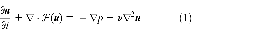

where


with the constraints
Velocity correction method and temporal discretization
The velocity correction method combined with discontinuous Galerkin (DG) has been investigated by several works, including Hesthaven and Warburton, 11 Ferrer et al., 4 and Emamy et al. 7 Here, the fixed semi-explicit dual-splitting schemes are used to solve equations (1) and (2). Within this scheme, the INS equations are split into three distinct substeps which can be solved successively.
In the first substep, equation (1) is advanced using Adams–Bashforth time scheme with the nonlinear convection term treated explicitly

where
The second substep is pressure projection, in which the intermediate velocity is updated with the following equation

By projecting the velocity into weakly divergence free space, equation (6) turns into a Poisson equation for pressure at time

Specially, Neumann boundary conditions should be applied on

where

The final substep takes the viscosity into consideration and solves an implicit Helmholtz equation

Spatial discretization
DG and CG space
The space discretization deployed here is based on the combination of DG and standard CG method. This choice benefits from the stability of DG on handling convection term and efficiency of CG in solving the projection step.
The computational domain denoted by

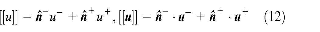
The discontinuity of variables across adjacent cell faces may be expressed in similar formulation
To discrete in either continuous or discontinuous formulation, approximate solution

where

The choice of basis function is critical to space discretization. Here, the discontinuous and continuous basis function space is defined as

Following the method introduced in the work by Hesthaven and Warburton,
11
a set of hierarchical orthogonal basis is constructed by
Till now, we have an arbitrary order modal basis to represent the continuous or discontinuous function space. Although they are equivalent mathematically, the nodal basis is more favorable for space discretization for its convenience on handling boundary conditions. By providing the position of the nodal point, namely, Legendre–Gauss–Lobatto (LGL) quadrature points, the Lagrangian nodal basis can be derived from a modal basis. The transformation matrix between nodal and modal basis is called Vandermond matrix. LGL points are essential to keep the matrix well conditioned. Since the basis functions talked above are defined on each cell piece-wisely, they maintain discontinuity on cell interfaces. However, to satisfy
Variational form of discretization terms
Convective term
The convective term is in the momentum equation of the first substep. To increase stability for convection dominant flow, upwind DG method is used in the discretization of the convective term. Integrating by parts and using Lax–Friedrichs flux, the discrete formulation of the convective term can be derived as

where

Laplacian term
The Laplacian term in pressure projection step is discretized with CG method. Since variables are continuous across interfaces in the framework of CG, flux integration can be ignored for internal faces. The variational formulation is given as

where the pressure gradient on Dirichlet boundaries is calculated by equation (8). Reference values on Neumann conditions are imposed by altering discretized linear system explicitly.
In the third viscosity substep, Laplacian term is discretized within DG framework using internal penalty formulation following methods used by Hesthaven and Warburton,
11
which helps to avoid spurious jumps on interfaces and provides sufficient stabilization. For the

The penalty parameter
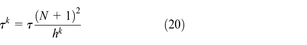
in which
Gradient and divergence term
According to the work by Fehn et al., 9 the implementations of gradient and divergence term are critical to avoid small time instability. So, we shall illustrate the discretization of these two terms in detail, and show the differences between various methods.
The implementation of our DG-CG method is similar to the work by Botti and Di Pietro. 10 The gradient of pressure is calculated explicitly by derivative of basis function as shown in equation (21).

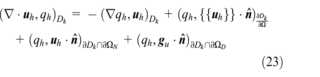
Divergence of intermediate velocity uses integration by parts to include information from neighbor cells and boundary conditions, as shown in equation (22). This is to make the divergence term consistent with viscosity substep (equation (19))

The approximation of velocity on cell interfaces are evaluated by central flux

Imposing the boundary conditions illustrated in equation (17), the final formulation of divergence term is derived as
where
To give a more direct illustration of the implementation, the corresponding pseudocode in Matlab style for two-dimwnsional (2D) case is provided as follows:
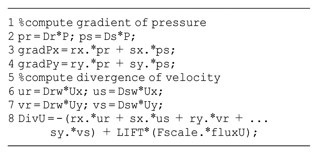
In the pseudocode,
To examine the small time stability of DG-CG method, it is necessary to find a reference. The method by Hesthaven and Warburton 11 is a widely used pure DG method, but reported to be unstable for small time step in the work by Krank et al. 5 In HW’s method, both pressure gradient and velocity divergence are calculated explicitly, as shown in the following equation

The corresponding pseudo-code is listed below.
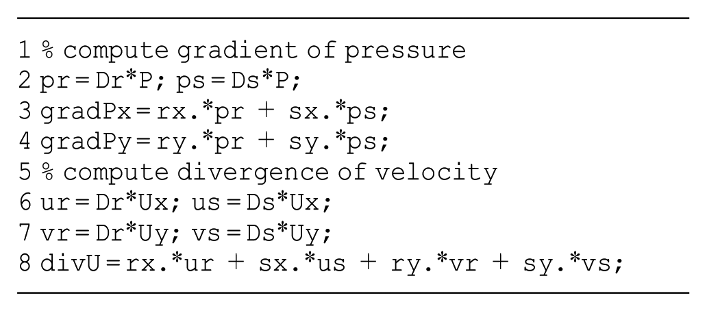
As argued by Fehn et al., 9 the DG formulation of velocity divergence and pressure gradient term are the essential reasons for the small time instability. He recommends that integration by parts coupled with a suitable definition of boundary conditions should be used to keep stable and robust. The major difference from HW’s method is performing integration by parts for both pressure gradient and velocity divergence, which are consistent with schemes used in pressure projection and velocity correction substeps. In Fehn’s method, the discretization of velocity divergence is almost the same as the one used in our DG-CG method (equation (22)). But the pressure gradient term is different, which is discretized with integration by parts. We can obtain the variational formulation as

where

It should be noted that the pressure in DG-CG method is continuous across element interfaces. That is to say, applying integration by parts for pressure gradient term in DG-CG method will not bring much difference. In the view of pressure gradient and velocity divergence, the DG-CG method is nearly the same as the one used in Fehn et al. 9 As Fehn claims that not applying integration by parts will lead to small time instability for pure DG method, one may ask whether the same phenomenon will happen in our mixed DG-CG method. Thus, we will also examine the DG-CG method using inconsistent velocity divergence scheme, as illustrated in equation (24). This method will be short for DG-CG_I in the later context.
Numerical results
The solver is implemented within the open-source framework HopeFOAM, 13 which aims at bringing high-order methods to official OpenFOAM based on second-order finite volume (Jasak et al., 14 Yang et al., 15 Wang et al. 16 ). The released HopeFOAM-0.1 provides high-order DGM, as well as high-order curved mesh, making it capable of achieving accurate space discretization. It inherits the user interfaces from OpenFOAM, including domain specified language, control dictionary, and boundary condition settings. Thus, developing high-order solver and cases within HopeFOAM is relatively convenient.
The linear system solver in HopeFOAM is based on PETSc, 17 which is a library intended for solving large-scale scientific applications modeled by partial differential equations. It supports most of the commonly used linear solver and preconditioner for the sparse matrix. In the following context, the ilu preconditioned GMRES Krylov iterative method is used.
Pearson vortex
Pearson vortex simulation is an unsteady INS problem and frequently used to demonstrate the small time step instability. The solution is constituted by making temporal derivatives in momentum equation equal with viscous term and non-linear convective term balance with pressure gradient. The analytical solution is given by

The computational domain is shown in Figure 1 enclosed by four inlet and four outlet boundaries. Dirichlet condition is enforced on inlets and Neumann condition on outlets for velocity, in which the boundary values are set by analytical solution. We choose viscosity

The computational domain of Pearson vortex simulation and boundary conditions.
Small time instability analysis
Since the small time instability is frequently reported on under-resolved cases, the simulation is performed on a mesh composed of 14 unstructured tetrahedral cells. Equal order polynomials are used for both pressure and velocity for all cases, with
The results in Figure 2 reproduce the phenomenon reported for Hesthaven and Fehn’s method. For the HW’s method, instabilities exist in all cases and the relative error increases dramatically at small time step size. For Fehn’s method, integration by parts in pressure gradient and velocity divergence terms successfully remedy the instability for velocity. The relative error of velocity reduces to a stable value, which is dominated by spatial error.

Relative
The equal order DG-CG and DG-CG_I methods show great stability at small time step for both velocity and pressure at all polynomial orders. Similar relative
It should be noted that the
Eigenvalue spectrum analysis
The eigenvalue spectrum analysis of the propagation matrix is performed to examine temporal stability of DG-CG method. Similar analysis has also been used in Leriche et al.
19
for spectral element collocation schemes and in Fehn et al.
9
for pure DG scheme. To perform this, the source term is discarded, harmonic boundary conditions are used for velocity, and the convective term is neglected. Then, the velocity

To compute

The max eigenvalues as a function of time step size are calculated on the problem defined in the previous subsection. Figure 3 shows the results of DG-CG method and pure DG by Hesthaven. For our DG-CG method, all eigenvalues are less than
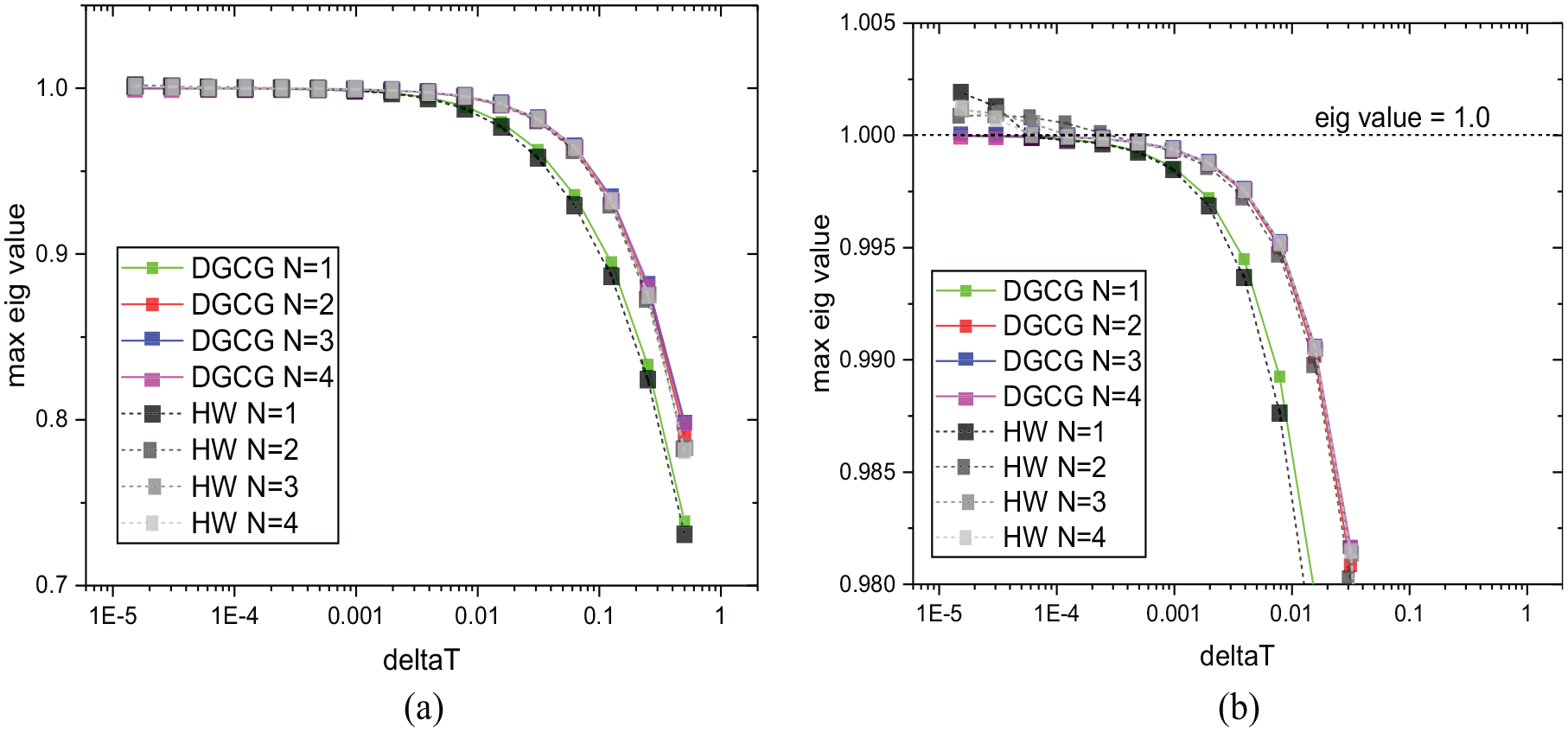
Maximum eigenvalue as a function of time step size: (a) original view and (b) enlarged view.
Spatial stability in low viscosity situation
In this section, the spatial stability of equal order DG-CG method in low viscosity situation is analyzed. The behavior of equal-order DG-CG method at high Reynolds number is what we care about. In addition, how to keep stable is quite important when we try to apply the DG-CG method.
This test is carried on Poiseuille flow case. In the Pearson vortex case, the viscosity term is set to balance with the convective term especially. Therefore, solving of pressure does not depend on viscosity. Thus, Pearson vortex is not suitable to investigate the instability caused by low viscosity. In Poiseuille flow, the viscous equals with pressure gradient term in the final steady state. Notably, the flow pattern of Poiseuille flow is common in computational fluid dynamics (CFD). This is a steady INS problem in two dimensions with an analytical solution
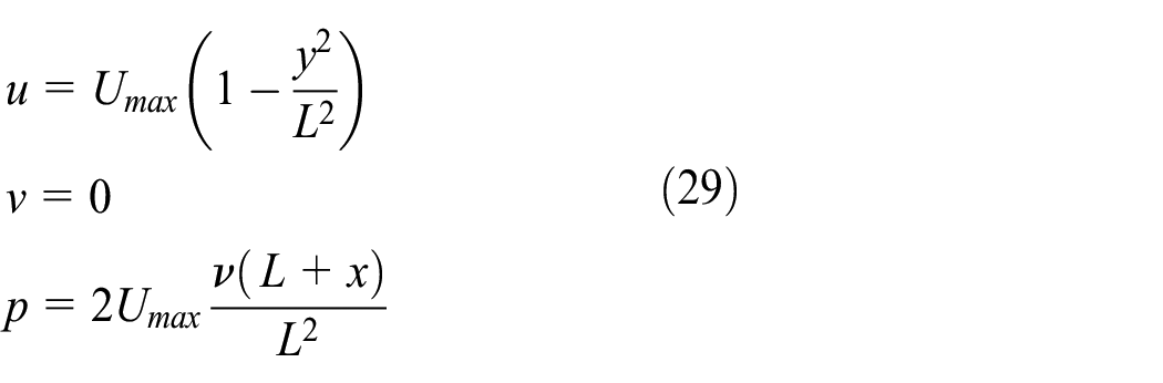
The computational domain
First, the simulations are carried out with
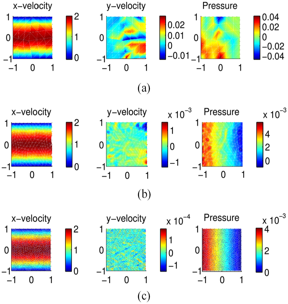
Simulation results of Poiseuille flow under different mesh scales, including (a)
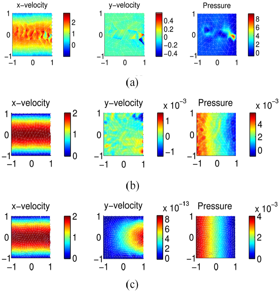
Simulation results of Poiseuille flow under different polynomial orders, including (a)
Then, various time step sizes and dynamic viscosities are also taken into consideration. The relative
Relative

NAN means this case cannot get convergent in the simulation.
At last, we can conclude that equal order DG-CG method may fail for high Reynolds number cases under low spatial resolution. But with sufficient mesh resolution and polynomial order, coupling with proper time step size (CFL condition), accurate simulation results can still be achieved.
3D Beltrami flow and convergence test
This 3D case is developed by Ethier and Steinman
22
for benchmarking purposes, and is a counterpart of 2D Taylor vortex problem. This problem is defined on domain

Here, the parameters are defined as dynamic viscosity
The point-wise error in

Point-wise error in
To reduce the influence of error introduced by spatial discretization, the polynomial order is set with

Results of 3D Beltrami flow simulation: (a) Temporal convergence rate of velocity and pressure using J=1 and J=2 and (b) Snapshot of velocity magnitude at T=1s.
Cavity flow
Here, we consider two-dimensional lid-driven cavity flow with relative high Reynolds number. The computational domain is a unit square. Upper bound (the lid) is enforced with a constant velocity
Figure 8(a) shows the streamline of steady-state cavity. Two vortices appear at the bottom corner, which is consistent with the literature. The profile of x and y components of velocity along vertical and horizontal center line is drawn in Figure 8(b). The simulation results (the lines) fit well with the reference value (dots). 23 With special care on the mesh resolution and discretization order, DG-CG method can simulate relative high Reynolds problem and keep stable.

Results of lid driven cavity flow on mesh with 3606 cells on
3D laminar flow past cylinder
This is a very challenging case with unsteady time-varying inflow profile. As a simplification of practical applications, lots of papers have used this case to verify the 3D simulation accuracy of CFD code. For the benchmark problem, a cylinder locates at the middle line of a channel, while no-slip boundary conditions are employed on the walls. The detailed geometry configuration can refer to Schäfer et al. 24 and John 25 The inlet velocity is set with
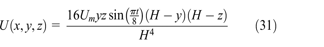
where

Snapshot of velocity magnitude for 3D laminar flow past cylinder using DG-CG method with
The maximum drag coefficient and minimum lift coefficient are major comparing criteria for this case. Results obtained by DG-CG and pure DG method under different polynomial orders are listed in Table 2. Accurate results are gained under both methods according to the reference values in Bayraktar et al.
26
It is worth to mention that results by our high order methods with
Maximum drag coefficient and minimum lift coefficient obtained by DG-CG and pure DG method under different polynomial order.
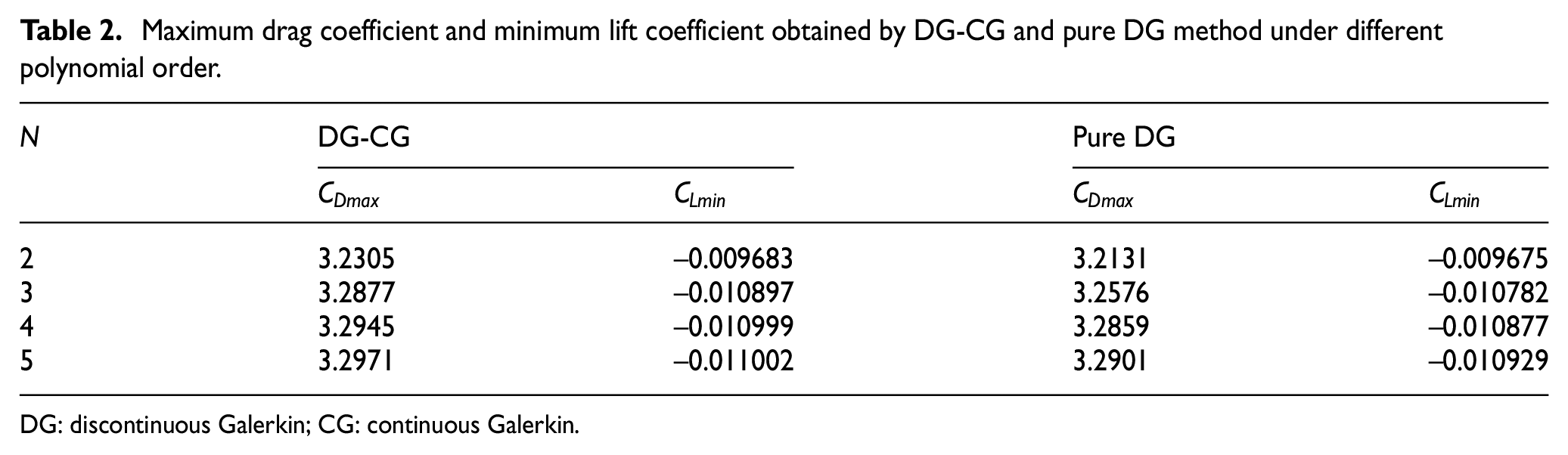
DG: discontinuous Galerkin; CG: continuous Galerkin.
Performance evaluation
DG method is preferred for its high-order convergence rate, stability, and high parallel efficiency while coming along with the disadvantages of extraordinary computation and memory overhead. This has been a major factor in obstructing its spread and application on complex problems. In the splitting method, solving of pressure takes up the major part of computational overhead. The solver with discontinuous velocity and continuous pressure has been examined to achieve high-order spacial convergence rate in previous sections. Moreover, pressure discrete by CG has the potential to be more efficient comparing to the discontinuous method. In this section, the performance of equal order DG-CG and pure DG method are analyzed under ilu preconditioned GMRES solver with the Pearson vortex case. The test ends at final time
The performance statistics of DG-CG and pure DG method are collected in Table 3, including the iterative number (n_it), computational time, and the number of degree of freedom (nDof) for each substep. Notation “pressure-cg” indicates the substep of solving pressure in DG-CG method, “pressure-dg” is a similar substep in pure DG method, and “velocity-dg” is the substep of solving velocity correction in both methods. Similar to the LU direct solver cases, DG-CG method has fewer Dofs and need less iterative steps to get convergence comparing to pure DG method. The speedup reaches up to 4 times at 896 test case while 6 times at 3584 test case, which is more significant at high-order scenario.
The ilu preconditioned GMRES solver profiling for DG-CG method and pure DG method.

DG: discontinuous Galerkin; CG: continuous Galerkin; nDof: number of degree of freedom.
Conclusion
In this article, we analyzed in detail the stability of the splitting method with discontinuous velocity and continuous pressure. Results are also compared to pure DG method by Hesthaven and Warburton
11
and Fehn et al.
9
For the small time step size problem, we first reproduce the instability with HW’s method on the simulation of Pearson vortex, while our DG-CG method remains stable at the same settings. As the time step size decreases continuously, the relative
In the work of Botti and Di Pietro, 10 the accuracy and performance of high-order polynomial are not discussed, where the highest pair is DG(3)-CG(2). In the stability analysis, we numerically show that higher polynomial order can lead to a more robust scheme in low viscosity situations. By the example of 3D Beltrami flow, up to sixth-order spatial convergence rate and second-order temporal convergence rate have been demonstrated. The cavity case is run on relative high Reynolds number flow condition, which confirms the stability of DG-CG method. At last, we check out the performance of DG-CG method at high polynomial order comparing with pure DG. Results show that DG-CG method is more efficient than pure DG method, to be specific, a speedup of 2.5 to 6 times on ilu preconditioned GMRES solver, which meets our initial expectation to develop mixed DG-CG solver.
Footnotes
Handling Editor: Roslinda Nazar
Declaration of conflicting interests
The author(s) declared no potential conflicts of interest with respect to the research, authorship, and/or publication of this article.
Funding
The author(s) disclosed receipt of the following financial support for the research, authorship, and/or publication of this article: This work was funded through the National Natural Science Foundation of China (Grant No. 61872380, 61802426), National Key Research and Development Program of China (No. 2016YFB0201301), and Science Challenge Project (No. TZ2016002).