Sage Journals: Discover world-class research

Abstract

This article proposes a deep learning technique for the prevision of the geometric accuracy in single point incremental forming. Moreover, predicting geometric accuracy is one of the most crucial measures of part quality. Accordingly, roundness and positioning deviation are two indicators for measuring geometric accuracy and presenting two output variables. Two types of artificial intelligence learning approaches, that is, shallow learning and deep learning, are investigated and compared for forecasting geometrical accuracy in the single point incremental forming process. Therefore, the back-propagation neural network with one hidden layer is selected as the representative for shallow learning and deep belief network and stack autoencoder are chosen as the representatives for deep learning. Accurate prediction is closely related to the feature learning of single point incremental forming process parameters. The following six parameters were considered as input variables: sheet thickness, tool path direction, step depth, speed rate, feed rate, and wall angle. The results of these studies indicate that deep learning could be a powerful tool in the current search for geometric accuracy prediction in single point incremental forming. Otherwise, the deep learning approach shows the best performance prediction with shallow learning. In addition, the deep belief network model achieves superior performance accuracy for the prediction of roundness and position deviation in comparison with the stack autoencoder approach.

Keywords

Single point incremental forming geometric tolerancing deep learning supervised learning unsupervised learning deep belief network stack autoencoder

Introduction

Single point incremental forming (SPIF) is an indispensable manufacturing process for customized production with high flexibility and rapid prototyping of sheet metal parts.¹ SPIF is a process of plastic deformation of the sheets.² The sheet forming is determined by a forming tool (hemispherical end or ball) controlled by a computer numerical control (CNC) milling machine and generating a trajectory defined by a computer-aided design (CAD)/computer-aided manufacturing (CAM) software.³ SPIF is endowed with several advantages over other conventional sheet forming processes, such as the ability to manufacture complex shapes and low production costs.⁴ Nevertheless, the main drawbacks of such process consist in the high production time and the limit of the geometric accuracy pertaining to the finished part.

Manufacturing quality prediction model has been developed using various data-driven techniques, to monitor the quality in advance, as an effective measure.⁵ Regarding sheet metal forming process, the geometrical accuracy of parts is the most important aspect with respect to the quality of benchmark geometry. However, the dimensions and geometrical inexactitudes have greatly limited the industry take-up of SPIF.⁶ As geometrical inexactitudes significantly limit the development of sheet metal forming, numerous research works have been developed to obtain better geometric accuracy. In fact, the design tolerance specifications, the design dimensions, and the process errors are closely interrelated. Besides, the knowledge of SPIF process errors with respect to design dimensions and tolerance specifications allow an optimal choice of SPIF parameters.

Numerous research works have been conducted to study the effect of geometries pertaining to forming tools. Maqbool and Bambach⁷ have determined that the relationship between the geometrical accuracy and process parameters of SPIF, based on how the contributions of three deformation modes (membrane stretching, bending, and through-thickness shear), varies by changing the process parameters. Indeed, the results showed that geometrical accuracy is very dependent on tool diameters and tool step-downs, and the SPIF process is a combination of three modes of forming. Lu et al.⁸ have proposed a novel model predictive control (MPC) approach to obtain improved geometric accuracy in SPIF. The MPC approach is founded on the control and optimization of the toolpath, by optimizing the step depth at each forming step. Furthermore, such a method has been applied in two incremental point forming (TIPF).⁹ Hamouche and Loukaides¹⁰ have identified the metal forming fabrication process as an integral part of the final geometry using an automatic learning approach. This approach makes it possible to automate and improve the leaf forming selection process. The results show that the best-performing classifier used a deep convolutional neuron network with an accuracy of 89%. Jaremenko et al.¹¹ have proposed a semi-supervised classification approach for the detection of the onset of localized necking in sheet metal forming of AL AA5182 using the deep learning approach. The results achieved using the proposed approach are consistent with the results of the time-dependent forming limit curve of the “line-fit” method.

According to the previous literature, several attempts have been made to control and optimize the geometric accuracy of the SPIF process. The main methods used incorporate modifying the process configuration or using temperatures to lower the flow stress and ductility enhancement, which results in compensating the undesirable springback effect.¹² On the contrary, several authors have studied the effect of various parameters, pertaining to the SPIF process, on the characterization of the geometric accuracy by predicting artificial intelligence (AI) and expert system. Taherkhani et al.¹³ have studied dimensional accuracy, surface quality, and production time using the group method of data handling (GMDH) in artificial neural networks (ANNs). Tool diameter, tool step depth, sheet thickness, and feed rate are considered as process parameters, which characterize the model. After the evaluation of the model accuracy, a genetic algorithm technique is used to optimize single- and multi-objective models. Ambrogio et al.¹⁴ have proposed a hybrid method to study the incremental forming limit. A neural network approach configured by Taguchi’s method is employed to predict the deformation limit depth. The following two different ANN algorithms are used: Levenberg–Marquardt (LM) and error back-propagation (EBP) algorithms. The results obtained indicate that the LM method is more efficient than the EBP method. Thus, Khan et al.¹⁵ have proposed an intelligent process model (IPM), which is a generalized classification-based model for the generation of corrected coordinate clouds to predict springback. Mulay et al.¹⁶ have proposed ANN implementation for the prediction of the average surface roughness (R_a) and maximum forming angle (Ø_max) of AA5052-H32 material. In fact, they used the LM algorithm for two different ANN structures (4-n-1 and 4-n-2). The result shows that the (4-n-2) structure can predict the outputs (R_a and Ø_max) more efficiently than the (4-n-1) model.

Multivariate adaptive regression splines (MARS) models are used to predict the geometric accuracy in the SPIF process. Behera et al.¹⁷ have proposed a set of free-form geometric shapes to study the dimensional inaccuracies of grade 1 titanium sheet part. They have proposed the MARS models to predict springback. Various geometric features, identified by using mesh techniques such as borders, surfaces, planes, and ribs, have been generated and trained by the MARS models. Indeed, individual STereo-Lithography (STL) files are created for each feature. The regression models are generated and trained using STL files, and a new tool path is generated. The results revealed that the compensated tool paths can minimize the average dimensional errors, which were about ±0.4 mm.

In this article, we propose a shallow learning and deep learning methods for the geometric accuracy prediction of SPIF. Accordingly, the aim of this study is to present and evaluate the performance of back-propagation neural network (BPNN), deep belief network (DBN), and stacked autoencoder (SAE) approaches as roundness and position deviation (PE) prediction methods. Correspondingly, the following two geometric accuracy indices are selected: roundness and positional deviation. Each method was applied to forecast each geometric accuracy parameter. The comparison of the performance of the learning approaches to investigate the feature learning capacity pertaining to the two models was conducted.

Scope of research

The geometrical accuracy of a part obtained by means of SPIF depends on the process parameters, such as forming tools and material behavior. These two factors have been studied in the most recent research via different methodologies, that is, finite element (FE) simulation, ANN, and machine learning (ML). This article is an extension of the study pertaining to the geometric accuracy of the SPIF process. The following two geometrical specification factors that designate the geometrical accuracy have not yet been studied: roundness deviation and PE. In addition, the prediction of two factors in terms of six viable factors is determined by deep learning. To the best of our knowledge, a few studies in the literature have reported the applications of geometric accuracy prediction using deep learning. Therefore, deep learning technique can provide a possibility for geometric accuracy prediction. The accurate prediction is closely related to the feature learning about the SPIF process.

This article incorporates two major parts, that is, the first, which is the distorted phase of the data collection method, and the second phase, which is the shallow learning and deep learning methods for SPIF prediction.

Experimental design and data processing

SPIF design

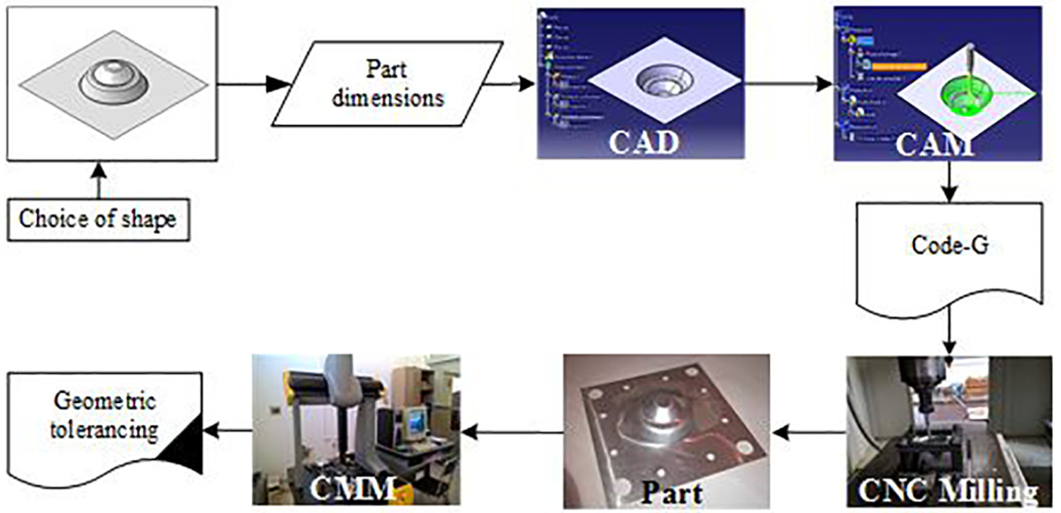
The geometrical accuracy of a part obtained by SPIF depends on several phenomena, such as the deformation mechanisms, the residual stresses,⁶ and springback.¹⁸ Depending on the condition and experimental setup as well as the complexity of the process, to conduct a test series of the SPIF, four steps were followed. First, we designed the shape of the part (CAD). In this work, a double truncated cone is chosen as benchmark geometry. The shape is termed as two forming angles, which are changing forms of 40° and 60°. The first truncated cone consists in the initial base, characterized by a 100 mm diameter and a 20 mm height. The second truncated cone is characterized by a 60 mm diameter and a 15 mm height. The part was manufactured using aluminum sheets (AA1050) with variable thicknesses of 0.6 and 0.8 mm.

Second, the machining phase generated the program of the forming tool (CAM). This step was carried out by using CAD/CAM software (CATIA). After CAM simulation, the NC program was transferred to a vertical milling machine (SPINNER VC 650), equipped with a steel tool, with a diameter of 10 mm, to produce the desired parts. Then, once the manufacturing process was completed, the control of the parts obtained was determined using a coordinate measuring machine (CMM). Besides, two geometrical specifications determined the roundness and PE. The measurements of roundness and PE were performed via a DEA GLOBAL CMM, coupled by a three-dimensional metrology module PCDMIS, with a measurement accuracy equal to 3.5 μm. Finally, a measured value report was generated by CMM, including the roundness and PE of each selected point.

The approach steps utilized in the SPIF are shown in Figure 1.

Figure 1.

Experimental methodology.

Tool path strategy is a key step in terms of incremental forming process. The choice of the tool path has an influence on the geometric accuracy. When manufacturing the parts, two different tool path strategies were used. These latter adopt a constant depth of pass; however, the movement direction is different. The first one possesses only one direction of movement and the second has an alternating direction, as indicated in Figure 2.

Figure 2.

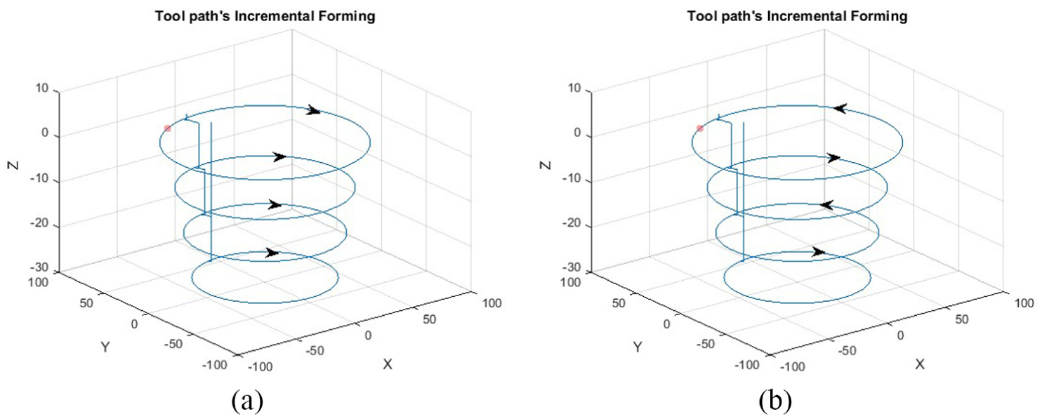
Strategies of tool path: (a) single-direction tool path and (b) alternating-direction tool path.

Data collection and analysis

In this work, the circular features defined the two truncated cone parts. The roundness and positioning tolerance controlled each circular feature independent of each other. The roundness deviation is the radial distance between the CAD and measured profile (Figure 3), containing the profile of the surface at a section perpendicular to the axis of the part. The PE is the radial deviation calculated between the CAD and the measured position. The CMM performed 30 complete cycles of circular movements. Each cycle consisted of 360° with measurement points all 10°. The vertical distance between each cycle was set at 1 mm.

Figure 3.

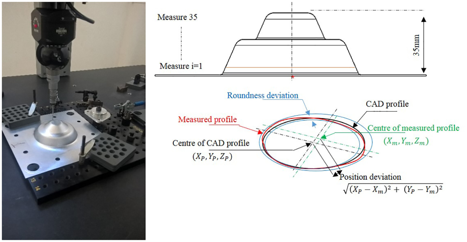
Measurement of roundness and position deviation.

To obtain the roundness and PE, experimental tests were performed. In the experimental plan, the process parameters, that is, strategy tool path, incremental step size, spindle speed, feed rate, and the forming angle, were varied at two levels. The input parameters and their levels are shown in Table 1.

Table 1.

Input parameters and their levels.

Notations	Factors	Unit	Levels
Δz	Vertical increment depth	mm	0.25	0.5
F	Feed rate	mm/min	500	1000
N	Speed rate	r/min	1500	3000
Th0	Sheet thickness	mm	0.6	0.8
A	Forming angle	Degree	40	60
TPS	Tool path strategy	–	Single	Alternating

TPS: tool path strategy.

In this section, all the measures from each parameter were grouped, and then the four groups were compared in order to evaluate their impact in geometrical accuracy. The box plots were used for graphical comparisons between database, to investigate roundness and position variations for the different forming angles. The box plot in Figure 4 displays the differences in test scores across two geometric specifications in SPIF.

Figure 4.

Box plot of roundness (a) and position deviation (b).

Roundness deviation was overexpressed in two forming angles (40° and 60°). A remarkable difference was detected between forming angles 40° and 60° in roundness deviation. This suggests that the forming angle has an important effect on the roundness. Although there is a visible difference between the median for the forming angles 40° and 60°, score difference is relatively small compared to the standard deviation for each forming angle.

For PE, the median of both parameters was the lowest in the forming angle of 40°, and a gradually increasing trend was observed from the forming angle of 60°. Besides, the forming angle of 40° had a very low standard deviation, while the highest deviation was observed in the forming angle of 60°. We can conclude that the forming angle effect was greatly significant to the geometric accuracy in the SPIF process.

The final database contains six input variables (thickness sheet, tool path strategy, step depth, speed rate, feet rate, and forming angle) and two output parameters (roundness and position deviation). Furthermore, this database is learned by the shallow and deep learning techniques. Two different deep learning approaches and shallow learning method were used and explained in the next section.

For the training phase, we have used 70% of the dataset and the remaining are used for the test phase.

Methodologies

BPNN

Recall that our problem is to determine the quality parameters from the process inputs (section “Experimental design and data processing”). Due to the nonlinearity of this problem, a BPNN is used to predict these parameters (values of the roundness and PE) for different possible situations and several input parameter variations. Moreover, a BPNN can be considered as a black box and consequently the planner can use it in a very simple way without a deep knowledge of its theoretical fundamentals.¹⁹ The general neural network architecture is given in Figure 5.

Figure 5.

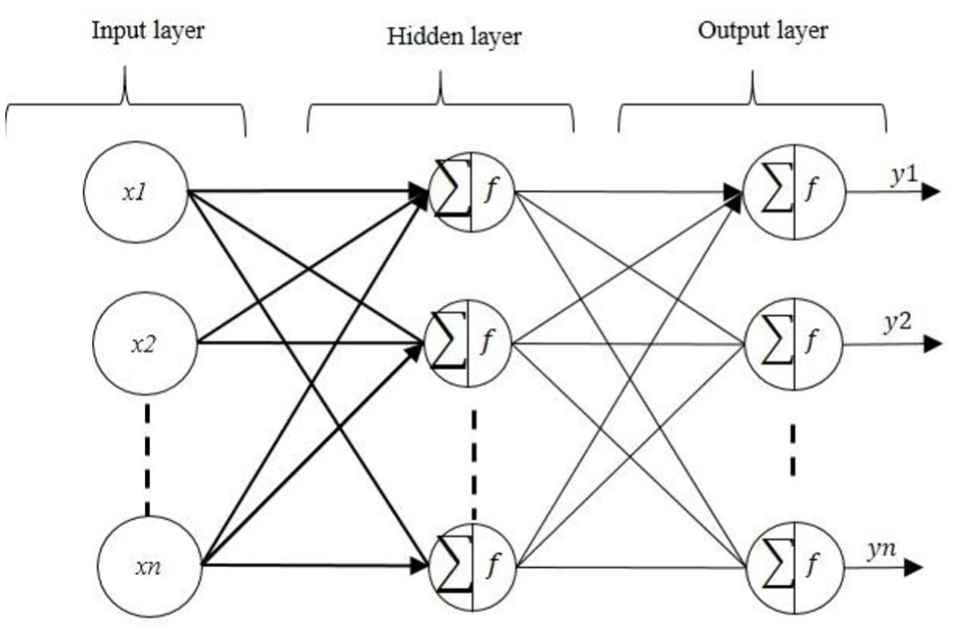
Architecture of BPNN.

Deep learning method

Deep learning is an important method for AI that enables improving the performance of algorithms by learning through the deep representations of the given dataset. The structure of deep learning algorithm consists of one input layer, several hidden layers to extract the deep features from the input layer, and one output layer for inference.²⁰ Deep learning is relatively a new paradigm of AI technique, and it was proposed by Hinton et al.²¹ Deep learning has improved the performance of algorithms by learning through the deep representations of the given dataset. The main credit of deep learning is the automatic feature extraction of complex data representations at high levels of abstraction.²² It has been successfully applied to a large number of fields, such as fault diagnosis,^23–25 pattern recognition,^26,27 and time series forecast.^28,29

This article aims chiefly at evaluating the merits of using new deep learning models for the prediction of SPIF data. In the next section, two deep learning approaches are introduced and investigated for the prediction of the geometric accuracy of SPIF, including the SAE and the DBN.

SAE

A basic autoencoder (AE) is a deep learning structure model, incorporating the following three layers: the input layer that represents inputs, the hidden layer that corresponds to learned features, and the output layer with the same dimension of the input layer that stands for reconstruction (Figure 6(a)). An original input is reconstructed at the output, going through an intermediate layer (hidden layer) with reduced number of hidden nodes. The AE training process consists of the following two steps: “encoder” and “decoder.” In the encoder step, the input and hidden layers construct the encoder network responsible for transforming the original inputs into hidden representation codes. In the decoder step, the hidden and output layers form the decoder network responsible for reconstructing original input data from the hidden representation codes.

Figure 6.

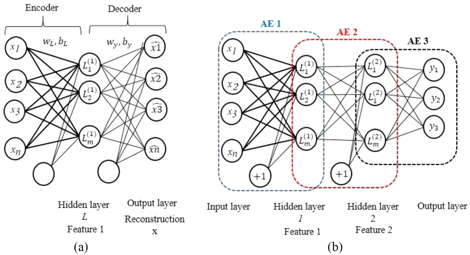
(a) The structure of autoencoder (AE) and (b) the structure of SAE in three hidden layers.

Hence, the encoding process is written as follows

L_{n} = f (w_{L} x_{n} + b_{L})

(1)

where $w_{L}$ is the weight matrix of encoder and $b_{L}$ is the bias vector.

The decoding process is as follows

Y_{n} = g (w_{Y} L_{n} + b_{Y})

(2)

where $w_{Y}$ is the weight matrix of the encoder and $b_{Y}$ is the bias vector.

To train the AE and determine the optimized parameters, the error between X and Y needs to be minimized

\underset{w_{L}, w_{Y}, b_{L}, b_{Y}}{\arg} min [error (X, Y)]

(3)

SAEs, in order to boost the performance of deep learning, were originally proposed in the study Bengio et al.³⁰ SAEs can be defined simply by introducing several hidden layers between the input layer and the output layer (Figure 6(b)). Therefore, the final reconstruction x is obtained through progressive abstraction levels.

DBN

DBN was proposed by Hinton et al.²¹ to demonstrate MNIST handwriting recognition task and verify the superior to feedforward neural networks.²⁰ It is an algorithm useful for dimensionality reduction, classification, and regression. DBN is based on sequence training with the restricted Boltzmann machine (RBM) approach to the initial weight matrix of DBN. An RBM is composed of two different layers of units, with weighted connections between them. It consists of one layer of visible node neurons, one layer of hidden units, and corresponding bias vectors: Bias a and Bias b. Connections between nodes are bidirectional and symmetric (Figure 7(a)). ν and h denote the state of the visible layer and hidden layer, respectively, and w is a weight matrix, connecting the visible and hidden neurons.

Figure 7.

(a) Structure of RBM and (b) structure of DBN.

Given the parameters set $θ = {w, a, b}$ , the joint probability distribution $P (v, h; θ)$ and energy function $E (v, h; θ)$ are described as

P (v, h; θ) = \frac{1}{Z} e^{- E (v, h; θ)}

(4)

E (v, h; θ) = - \sum_{i = 1}^{n} a_{i} v_{i} - \sum_{j = 1}^{m} b_{j} h_{j} - \sum_{i = 1}^{n} \sum_{j = 1}^{m} v_{i} w_{ij} h_{i}

(5)

where Z is the partition function, described as

Z = \sum_{v, h} e^{- E (v, h; θ)}

(6)

A DBN is a graphical model, which learns to extract a deep hierarchical representation of the training data. It models the joint distribution between an observed vector x and l hidden layers $h^{k}$ as follows

\begin{matrix} P (x, h_{1}, h_{2}, \dots, h_{l}) = P (v | h_{1}) \\ P (h_{1} | h_{2}) \dots P (h_{l - 2} | h_{l - 1}) P (h_{l - 1} | h_{l}) \end{matrix}

(7)

P (x, h_{1}, h_{2}, \dots, h_{l}) = (Π_{k = 0}^{l - 2} P (h_{k} | h_{k + 1})) P (h_{l - 1} | h_{l})

(8)

where $v = h_{0}$ , $P (h^{k} | h^{k + 1})$ is a conditional distribution for the visible units conditioned on the hidden units of the RBM at level k, and $P (h^{l - 1} | h^{l})$ is the visible–hidden joint distribution in the top-level RBM. The RBM and DBN structures are presented in Figure 7(a) and (b), respectively.

The proposed model and performance criteria

To compare the deep learning approaches (SAE and DBN), an experiment was designed and conducted to obtain the SPIF data for the training and the testing of the forecasters used. The SPIF data and detailed description are available in section “Data collection and analysis.” The SPIF data exploit six input variables (thickness sheet, speed rates, feed rate, forming angle, tool path, and vertical increment depth) to predict the roundness and PE.

Deep learning algorithm is divided into two stages as follows: pre-training and ﬁne-tuning. In pre-training, an unsupervised learning algorithm is used to pre-train the network, layer by layer.³¹ In the SEA approach, the target output value of each AE is set as its input. An AE approximates an identity function of the input, in order to learn the reconstruction ability.³² On the contrary, DBN can be formed by several unsupervised RBMs, where each RBM’s hidden layer serves as the visible layer for the next, which leads to an unsupervised layer-by-layer learning procedure.³³ The approach settings were epoch, batch size, and momentum at 2000, 1, and 0, respectively.

After the pre-training stage, the network parameters are then fine-tuned by supervised learning methods. The deep learning network was learned with the back-propagation algorithm. The back-propagation algorithm consists in feeding forward the values to generate an output and calculate the error between the output and the target output, then propagating it back to the earlier layers in order to adjust weights and biases.³³ The more prevalent activation function is the sigmoid

f (x) = \frac{1}{1 + e^{- x}}

(9)

The back-propagation settings were epoch and batch size at 2000 and 12, respectively.

In total, 70% randomly selected datasets were used to train the neural networks and the remaining eight datasets (30%) were employed to test and verify the network. For convenience, serval models of the BPNN, SAE, and DBN are learned. The models include six input variables (sheet thickness, tool path strategies, step depth, speed rate, feed rate, and forming angle), two output parameters (roundness and Position deviation), two hidden layers for SAE and DBN approaches, and one hidden layer for BPNN, with a number of hidden node n=(1–15) in each hidden layer. The models are developed using the real manufacturing data of the SPIF process. All these data are normalized to avoid the neuron saturation and to facilitate model learning phase. The normalization operation is given by the following equation

Normalization = \frac{x - x_{\min}}{x_{\max} - x_{\min}}

(10)

where $x_{\max}$ and $x_{\min}$ are the maximum and minimum values of each vector.

To evaluate the performances of the shallow and deep learning methods, two evaluation measures are used in this study: mean absolute percentage error (MAPE) and root-mean-square error (RMSE). The equations of the criteria are defined as follows

MAPE = \frac{100}{N} \sum_{i = 1}^{N} | \frac{y_{act} - y_{predi}}{y_{act}} |

(11)

RMSE = \sqrt{\frac{1}{N} \sum_{i = 1}^{N} {(y_{act} - y_{predi})}^{2}}

(12)

where N is the number of data, $y_{act}$ is the experimental value (actual), $y_{pred}$ is the predicted value, and i is the ith observation and prediction.

Results

BPNN results

The (6-12-1) structure of the BPNN model has the best capability for all parameter outputs. It revealed the MAPE of the lowest train for the roundness deviation (5.008) and the PE (22.0737). The (6-12-1) structure also showed excellent predictability with least possible error. All results showed an excellent association between actual input and predicted output parameters.

After that, the BPNN was tested for serval combinations of 30% conducted experiments. The MSE and MAPE values are shown in Appendices 1 and 2. The generated BPNN model can predict the quality parameters with the higher certainty level for a new set of inputs.

SAE results

The SAE constructed a learning model using a training data. Six input variables (tool path strategy, thickness sheet, vertical increment, speed rate, feed rate, and forming angle) and two output data were used (roundness and position variation). The two outputs are trained separately, that is, one to the other. The performance of the model differed depending on the number of nodes constituting the SAE. The MAPE and RMSE according to the number of nodes are shown in Appendices 3 and 4. The smaller values of the MAPE and RMSE represent better prediction results. Considering all the obtained values of MAPE and RMSE, the best construction of an SAE is the (6-10-7-1) structure that exhibited the lowest MAPE and RMSE (1.4354 and 0.07439, respectively) in roundness deviation. The (6-11-10-1) structure showed the best MAPE and RMSE (2.2453 and 0.0238, respectively) in PE.

DBN results

As shown in Appendix 5 with respect to the case of roundness, the best structure of a DBN is (6-15-15-1), showing the lowest MAPE and RMSE (4.4231 and 0.0031, respectively) in roundness deviation. For case PE, the smaller values of the MAPE and RMSE are presented by the structure (6-12-7-1), which exhibited the best MAPE and RMSE (2.8589 and 0.0072, respectively) (Appendix 6).

Comparison studies and discussions

As discussed previously, the forming angle has a significant effect on the geometrical accuracy of parts formed by SPIF. In this context, shallow learning (BPNN) and two deep learning approaches (SAE and DBN) were used to predict geometric accuracy. The analysis based on the performance of the BPNN, SAE, and DBN for geometric accuracy prediction is presented in this section.

In addition to the training data, the number of hidden neurons has a decisive impact on the results. Since no methodology is known to determine the number of hidden neurons, an appropriate configuration must be identified by trial and performance criteria (MAPE and RMSE). Thus, the number of hidden neurons in each layer is model hyperparameters to specify. To determine the optimal number of hidden neurons, the sequential orthogonal approach was used. This approach consists in adding hidden neurons, one by one, until the prediction error is sufficiently low.

This approach is composed of two stages. In the first stage, one hidden layer structure of deep learning was used for the estimation of roundness and PE parameters with a variation in hidden neuron number from 1 to 15 nodes. In this case, we start a first hidden layer with one neuron, then increasing the number of neurons with a gradation of one neuron in each trial, until reaching a number of neurons equal to 15 nodes. In the second stage, a hidden second layer was added. The optimal number of hidden neurons in the first hidden layer remained optimal in the test suite, adding a second hidden layer, in which we increase the number of neurons by one neuron per trial. We conclude that the number of hidden neurons and the number of hidden layers have a significant impact on the performance.

To compare the proposed BPNN, SAE, and DBN, the number of trials is experimentally performed from serval independent trials and computed to perform results, as illustrated in Appendices 1–6, including the evaluation criteria indices (MAPE and RMSE). A smaller value of the MAPE and RMSE represents better prediction results and better performance of the model. Considering all the values of such indices, the predictors constructed by utilizing the roundness data perform better than those designed only by the positioning data. With respect to the number of hidden neurons and hidden layers, the results reveal that the DBN approach achieves a better performance.

First, the deep learning approaches (DBN and SAE) have a strong capacity for reconstructing the features of the manufacturing process data in SPIF. Second, the SAE approach has a weaker capacity for feature learning and regression, compared with the DBN approach (Table 2).

Table 2.

Comparison of the prediction performances using different approaches.

	Roundness deviation				Position deviation
	MAPE train	RMSE test	MAPE train	RMSE test	MAPE train	RMSE test	MAPE train	RMSE test
BPNN	5.0084	0.0121	9.4773	0.0136	22.0737	0.0303	29.12217	0.021568
SAE	1.4354	0.0744	3.2386	0.0730	2.2453	0.0238	1.0072	0.0201
DBN	4.4231	0.0031	9.0852	0.0037	2.8589	0.0072	1.4093	0.0069

MAPE: mean absolute percentage error; RMSE: root-mean-square error; BPNN: back-propagation neural network; SAE: stack autoencoder; DBN: deep belief network.

As a result, some values of the MAPE and RMSE in Appendices 1 and 2 are larger than those in Appendices 3 and 4. The predictors constructed by utilizing the DBN approach perform better than the SAE approach with the original data. To assess the performance of the resulting deep learning approaches, the percentage average accuracy of the predicted data is being recorded. The evaluation of the average accuracy of the two forecasting approaches is shown in Table 3. Accuracy when measuring roundness and position prediction was the highest at 97.8% and 96.7%, respectively, for the DBN approach. Besides, the existing SAE displayed low accuracies, 95.4% and 89.2%, respectively.

Table 3.

Percentage accuracy of predicting deep learning approaches.

	Roundness deviation (%)	Position deviation (%)
BPNN	83.33	83.33
SAE	96.7	89.2
DBN	97.8	95.4

BPNN: back-propagation neural network; SAE: stack autoencoder; DBN: deep belief network.

With respect to the prediction error distribution, simulations were conducted under the geometrical accuracy parameters. Figures 8 and 9 demonstrate the distribution error histograms of the approaches, designed in the two geometrical accuracy factors. The error distribution is represented by the prediction error values of the number pertaining to the prediction errors in different bins. It indicates that the mean of prediction error is close to zero, and the distribution is also close to the normal distribution.

Figure 8.

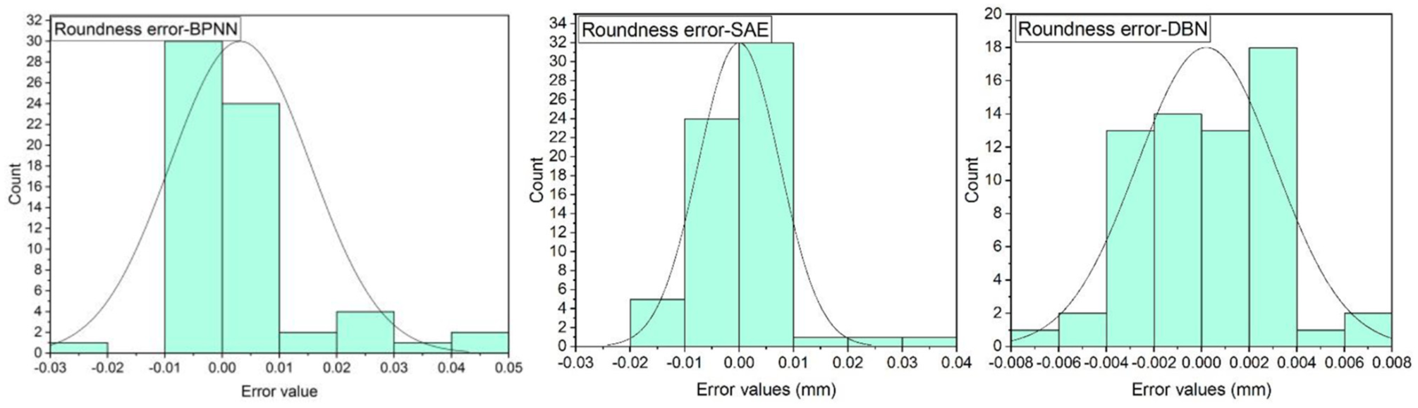
Distribution of error prediction in roundness deviation.

Figure 9.

Distribution of error prediction in position deviation.

The prediction error of PE by SAE and DBN approaches is provided in Figure 9. The proposed DBN approach generally achieves the best performance among all the compared SAE methods, and a strict ordering can also be observed.

The actual and predicted values of roundness and PE are illustrated in Figure 10. Given the vast amount of experiments performed, results are presented only for the best configurations and the best performances obtained in terms of MAPE and RMSE.

Figure 10.

Predicted results of the deep learning approaches: (a) by utilizing the roundness data, (b) by utilizing the position data.

It is worth mentioning that the number of the data used in this article is not very large. Although the DBN model is learned by small data in both experiments, it still displays excellent performances.

Conclusion

AI is critical for dimensional and geometric accuracy prediction in SPIF. Deep learning is a new research topic; however, it is very limited with respect to engineering application. In this article, a deep learning for roundness and PE forecasting is established, based on SAE and DBN approaches compared with shallow learning (BPNN). The proposed approaches are progressively trained in the pre-training phase and the fine-tuning phase, using the back-propagation algorithm.

The performance of shallow and deep learning to predict geometrical accuracy in the SPIF process is tested and compared in this article. The performances of the deep learning are better than those of the shallow learning in terms of the MAPE and the RMSE criteria.

Compared with the SEA and BDN approaches, the predicting error of the DBN proposed method in most cases achieves the highest accuracy as SAE. Furthermore, the proposed DBN approach achieves mean values of percentage accuracy in roundness and PE as 97.5% and 95.4%, respectively. Finally, the experiment results show that the proposed approaches can achieve similar performance to the shallow learning method. On the contrary, deep learning technique shows the best practicality in terms of implementation in the SPIF process.

Based on the findings, the contribution of this study is that the deep learning technique can be applied successfully for small data, and deep learning exhibits a better capability of predicting the geometric accuracy in the SPIF process compared with shallow learning.

Footnotes

Appendix

Appendix 6

MAPE and RMSE according to node number of the position deviation using the DBN approach.

Trial	Hidden layer 1	Hidden layer 2	MAPE (%) train	RMSE train	MAPE (%) test	RMSE test
1	1	0	25.8124	0.0372	23.889	0.0237
2	2	0	38.1608	0.0379	69.5387	0.0249
3	3	0	64.257	0.0371	11.0297	0.0292
4	4	0	40.6959	0.0362	11.4813	0.0227
5	5	0	21.586	0.0363	0.0016	0.0234
6	6	0	10.608	0.0385	0.0318	0.0254
7	7	0	54.056	0.0362	19.1291	0.0250
8	8	0	99.4034	0.0362	74.7749	0.0223
9	9	0	72.2298	0.0362	36.7827	0.0216
10	10	0	13.7087	0.0351	15.3392	0.0163
11	11	0	83.4674	0.0350	24.7107	0.0224
12	12	0	16.5899	0.0368	13.7078	0.0233
13	13	0	71.8336	0.0358	18.6294	0.0221
14	14	0	66.7521	0.0367	60.8623	0.0222
15	15	0	24.9515	0.0326	89.79	0.0224
16	12	1	10.5893	0.0367	8.8753	0.0325
17	12	2	7.9539	0.0303	5.3639	0.0220
18	12	3	19.4014	0.0210	4.3312	0.0168
19	12	4	31.2278	0.0150	32.0076	0.0179
20	12	5	12.9635	0.0121	4.1247	0.0131
21	12	6	3.4869	0.0100	11.7258	0.0856
22	12	7	2.8589	0.0072	1.4093	0.00698
23	12	8	5.539	0.0102	24.7856	0.0091
24	12	9	5.1301	0.0109	66.4162	0.0125
25	12	10	6.6556	0.0101	69.826	0.0086
26	12	11	16.0928	0.0085	54.8781	0.0082
27	12	12	7.6068	0.0078	14.6487	0.0082
28	12	13	25.7769	0.0081	3.831	0.0088
29	12	14	15.691	0.0096	39.2914	0.0093
30	12	15	5.159	0.0083	28.1466	0.0078

MAPE: mean absolute percentage error; RMSE: root-mean-square error; DBN: deep belief network.

Handling Editor: James Baldwin

Declaration of conflicting interests

The author(s) declared no potential conflicts of interest with respect to the research, authorship, and/or publication of this article.

Funding

The author(s) received no financial support for the research, authorship, and/or publication of this article.

ORCID iDs

Sofien Akrichi

Amira Abbassi

References

Mirnia

Shamsari

Numerical prediction of failure in single point incremental forming using a phenomenological ductile fracture criterion. J Mater Process Tech 2017; 244: 17–43.

Hirt

Ames

Bambach

et al . Forming strategies and process modelling for CNC incremental sheet forming. CIRP Ann: Manuf Techn 2004; 53: 203–206.

Ben Said

Mars

Dammak

. Numerical prediction of the ductile damage in single point incremental forming process. Int J Mech Sci 2017; 131–132: 546–558.

Fadhil

Thamir

Raheem

et al . Influence of forming angle on geometrical accuracy in single point incremental sheet metal forming (SPIF) process. Int J Mech Prod Eng Res Dev 2018; 8: 1135–1144.

Bai

Sun

Zeng

et al . A comparison of dimension reduction techniques for support vector machine modeling of multi-parameter manufacturing quality prediction. J Intell Manuf 2019; 30: 2245–2256.

Liu

et al . Study on step depth for part accuracy improvement in incremental sheet forming process. Adv Mat Res 2014; 939: 274–280.

Maqbool

Bambach

Dominant deformation mechanisms in single point incremental forming (SPIF) and their effect on geometrical accuracy. Int J Mech Sci 2018; 136: 279–292.

Kearney

et al . Model predictive control of incremental sheet forming for geometric accuracy improvement. Int J Adv Manuf Technol 2015; 82: 1781–1794.

Haibo

Michael

Chenhao

et al . Part accuracy improvement in two point incremental forming with a partial die using a model predictive control algorithm. Precis Eng 2017; 49: 179–188.

10.

Hamouche

Loukaides

EG.

Classification and selection of sheet forming processes with machine learning. Int J Comp Integ M 2018; 31: 921–932.

11.

Jaremenko

Ravikumar

Affronti

et al . Determination of Forming Limits in Sheet Metal Forming Using Deep Learning. Materials 2019; 12: E1051.

12.

Mohammadi

Vanhove

Bael

et al . Towards accuracy improvement in single point incremental forming of shallow parts formed under laser assisted conditions. Int J Mater Form 2014; 9: 339–351.

13.

Taherkhani

Basti

Nariman-Zadeh

et al . Achieving maximum dimensional accuracy and surface quality at the shortest possible time in single-point incremental forming via multi-objective optimization. Proc IMechE, Part B: J Engineering Manufacture 2018; 233: 900–913.

14.

Ambrogio

Filice

Guerriero

et al . Prediction of incremental sheet forming process performance by using a neural network approach. Int J Adv Manuf Technol 2011; 54: 921–930.

15.

Khan

Coenen

Dixon

et al . An intelligent process model: predicting springback in single point incremental forming. Int J Adv Manuf Technol 2015; 76: 2071–2082.

16.

Mulay

Ben

Syed

et al . Artificial neural network modeling of quality prediction of a single point incremental sheet forming process. Adv Sci Technol Lett 2017; 147: 244–250.

17.

Behera

Verbert

Lauwers

et al . Tool path compensation strategies for single point incremental sheet forming using multivariate adaptive regression splines. Comput-Aided Design 2013; 45: 575–590.

18.

Araújo

Silva

Montanari

et al . Evaluation of the dimensional accuracy in single point incremental forming. AIP Conf Proc 2013; 1567: 832–835.

19.

Abbassi

Akrichi

Yahia

NB.

Experimental study of drilling white Calacatta-Carrara marble using artificial neural approach. Adv Mech Eng. Epub ahead of print 13 March 2019. DOI: 10.1177/1687814019833579

20.

Bengio

Courville

Vincent

Representation learning: a review and new perspectives. IEEE T Pattern Anal 2013; 35: 1798–1828.

21.

Hinton

Osindero

Teh

YW.

A fast learning algorithm for deep belief nets. Neural Comput 2006; 18: 1527–1554.

22.

Maryam

Flavio

Taghi

et al . Deep learning applications and challenges in big data analytics. J Big Data 2015; 2: 1.

23.

Wang

Rui

et al . Bearing fault diagnosis method based on Hilbert envelope spectrum and deep belief network. J Vibroeng 2015; 17: 1295–1308.

24.

Chuan

René-Vinicio

Grover

et al . Fault diagnosis for rotating machinery using vibration measurement deep statistical feature learning. Sensors 2016; 16: E895.

25.

Jia

Lei

Lin

et al . Deep neural networks: a promising tool for fault characteristic mining and intelligent diagnosis of rotating machinery with massive data. Mech Syst Signal Pr 2016; 72: 303–315.

26.

Shan

Khalil-Hani

Bakhteri

Bounded activation functions for enhanced training stability of deep neural networks on visual pattern recognition problems. Neurocomputing 2016; 216: 718–734.

27.

Gan

Wang

Zhu

Construction of hierarchical diagnosis network based on deep learning and its application in the fault pattern recognition of rolling element bearings. Mech Syst Signal Pr 2016; 73: 92–104.

28.

Bai

Sun

Zeng

et al . A multi-pattern deep fusion model for short-term bus passenger ﬂow forecasting. Appl Soft Comput 2017; 58: 669–680.

29.

Kuremoto

Kimura

Kobayashi

et al . Time series forecasting using a deep belief network with restricted Boltzmann machine. Neurocomputing 2014; 137: 47–56.

30.

Bengio

Lamblin

Popovici

et al . Greedy layer-wise training of deep networks. Adv Neur In 2007; 19: 153–160.

31.

Schmidhuber

Deep learning in neural networks: an overview. Neural Netw 2015; 1: 85–117.

32.

Liu

Yang

. A flood forecasting model based on deep learning algorithm via integrating stacked autoencoders with BP neural network. In: Proceedings of the 2017 IEEE third international conference on multimedia big data (BigMM), Laguna Hills, CA, 19–21 April 2017, pp.58–61. New York: IEEE.

33.

Shah

Trivedi

. Optimizing back propagation parameters for anomaly detection. In: Proceedings of the IEEE—international conference on research and development prospectus on engineering and technology, Nagapattinam, India, 29–30 March 2013. New York: IEEE.