
Abstract
Artificial intelligence is one of the hottest research topics in computer science. In general, when it comes to the needs to perform deep learning, the most intuitive and unique implementation method is to use neural network. But there are two shortcomings in neural network. First, it is not easy to be understood. When encountering the needs for implementation, it often requires a lot of relevant research efforts to implement the neural network. Second, the structure is complex. When constructing a perfect learning structure, in order to achieve the fully defined connection between nodes, the overall structure becomes complicated. It is hard for developers to track the parameter changes inside. Therefore, the goal of this article is to provide a more streamlined method so as to perform deep learning. A modified high-level fuzzy Petri net, called deep Petri net, is used to perform deep learning, in an attempt to propose a simple and easy structure and to track parameter changes, with faster speed than the deep neural network. The experimental results have shown that the deep Petri net performs better than the deep neural network.
Keywords
Introduction
Encountering the needs for implementation, it often requires lot of relevant efforts to construct a learning structure. In order to make a full connection among nodes, the learning structure becomes complicated. It is not easy for developers to track the parameters changed inside. Therefore, this reason motivates us to provide a streamlined method to perform deep learning. In Shen et al.’s study, 1 the high-level fuzzy Petri net (HLFPN) toward machine learning has been successfully proved. The HLFPN model provides a faster, less-complex, and easier implementation method. Thus, this article aims to use the multilayer HLFPN to perform deep learning, in an attempt to propose a simpler structure, easier to track the parameters changed, and a faster architecture than the neural network (NN).2–6
The difference from the work by Shen et al. 1 is mainly the structural changes. The structure of the HLFPN model is different from the deep neural network (DNN) model because they both depend on the types of problems. 7 However, the DNN is a fixed structure, only fine-tuning the algorithm for each layer. 8 The HLFPN model is intended to solve this specific problem. First, write the predicate logic based on the problem. 9 Then, draw the structure according to the predicate logic and use the structure to perform machine learning. The advantages of this design for the problem can make the HLFPN model simpler and have no redundant nodes so as to decrease the complexity of the structure.
The proposed architecture is called deep Petri network (DPN). Similar to HLFPN, first, write the predicate logic based on the problem; then, draw the structure according to predicate logic and use this drawn structure to perform targeted deep learning because the design process makes the problem formulation have the advantages of the structure. DPN makes the structure simpler; and does not require redundant nodes to increase the complexity of the structure.10–13 Hence, the simpler structure can effectively improve the computational speed.
This study proposes a concept of “ring.” The DPN model was developed to simulate an NN model.14,15 It is formed layer by layer and is placed from left to right. Its structure is expressed in layers like a planet orbit. The transitions and places required by the predicate logic are placed layer by layer on the ring. Each node is linked to the core at the end, and the core determines whether or not the calculation result is done as expected. The concept of a core is to perform the unsupervised or supervised deep learning. Finally, the results of the core decision will be passed to the supervisor node at the outermost ring so as to correct the initial values of the entire system.16–19
The supervisor node located at the outermost ring makes the entire system become a complete loop, which makes the learning logic easier to be observed. Since the DNN does not show the graphical modification of the weights, which makes it difficult for the beginners to understand, the supervisor node can monitor the changes of each system to determine whether or not the modification of the attribution degree changes differently in the convergence direction.20–22 Thus, the stability and convergence speed of the system are further improved.
In section “Literature review,” the recent research of the NN is presented, listing a few common types of NN to show the difference between each other. Then, the core algorithm of the HLFPN model is introduced. The main ideas of unsupervised and supervised DPN models are proposed in sections “Unsupervised deep learning algorithm” and “Supervised deep learning algorithm,” respectively. The effects of DPN are all discussed in section “Main results.” Finally, section “Conclusion” presents the conclusion and future work.
Literature review
The NN models have been completely studied. Especially, almost all of the developing technologies want more automated and more intelligent functions in recent years. In other words, they need to be combined with artificial intelligence (AI) techniques, and the foundation of AI techniques is deep learning. It is now aimed at all types of the problems so that there are a variety of NNs to deal with a wide range of problems.23,24
Deep learning
Deep learning is a kind of machine learning. In general, it is based on NN, but the number of layers is more than the original NN. 25 It makes data sets through linear or nonlinear transform in many layers to extract the features of data sets. Deep learning contains many different types for different problems, which are DNN, recurrent neural network (RNN), convolutional neural network (CNN), and deep autoencoder (DA).26–28
NN categories
In this sub-section, some popular NN models are listed to make a difference among them and to discuss their advantages.
DNN
DNN is the most basic NN. It is a kind of structure inspired by the human brain. The architecture is a layer-by-layer structure. In addition to the input and output layers, the middle one is called the hidden layer. Although DNN is the architecture that has been widely used, it still has inevitable problems that are slower and heavier.
RNN
The characteristics of RNN are to use the past results to calculate the current output. 3 This memory-like concept is very suitable for the time-dependent fields, such as text mining, time series, and some other fields. Nowadays, RNN’s research direction is that the memory time needs to become longer or shorter. For example, the data sets from different times in the past were used to simultaneously calculate the current output.
CNN
CNN is a composite NN. In general, the architecture is a convolutional layer followed by a traditional fully connected layer. The main part better than DNN is that it is more efficient for multi-quadrant data processing. The function of the convolutional layer is the input-data filtering. Two different structures can process the data differently. First, it reduces the data complexity in the convolutional layer. Then, the data transmitted to the fully connected layer is relatively simple, in order to achieve the goal of speeding up.
DA
The concept of DA is a stack of multiple DNNs. The main data processing is intended to project high dimension to lower dimension and to process it. DA is characterized by the use of more cells in the input and output, while hiding the cells that have been less used to achieve the goal of acceleration. Although the projection of units will make some data lost, the speed-up effect achieved by compressing data still makes DA become a popular NN architecture.
HLFPN
The HLFPN 1 is defined as an eight-tuple HLFPN = (P, T, F, C, V, α, β, δ), where
P = {p1, p2, p3,…, pk} finite set of places.
T = {t1, t2, t3,…, tl} finite set of transitions. P ∪ T ≠∅.
F ⊆ (P × T)∪(T × P) called the flow relation and is also a finite set of arcs, each one representing the fuzzy set (i.e. fuzzy term) for an antecedent or a consequent; where the positive arcs (i.e. THEN parts) are denoted by
C = {X, Y, Z} finite set of linguistic variables, for example, X, Y, and Z, where X = {x1, x2x3,…, xn}, Y = {y1, y2y3,…, ym}, and Z = {z1, z2z3,…, zq}.
V = {v1, v2v3,…, v4} finite set of fuzzy truth values known as the fuzzy relational matrix between the antecedent and the consequent of a rule.
α: P→C association function, mapping from places to linguistic variables. α(pi) = ci, i = 1,…, I, where C = {ci} is a set of linguistic variables in the knowledge base (KB), and I is the number of linguistic variables in the KB.
β: F→[0, 1] association function, mapping from the flow relations to the fuzzy truth values between 0 and 1.
δ: T→V association function, mapping from transitions to fuzzy relational matrices.
Unsupervised learning
The unsupervised learning scheme has no feedback coming from the environment to show what the desired outputs of a network should be or whether they are correct. The network must train itself to capture any relationship of interest from the input data and transform the captured relationships into outputs.1,11
Supervised learning
Supervised learning is the task of adjusting a function that maps an input to an output based on example input–output pairs. It infers a function from the labeled training data including a set of training examples. In the supervised learning, each example is a pair of input object and the desired output value. A supervised learning algorithm analyzes the training data and produces an inferred function, which can be used for mapping new examples. 2
Unsupervised deep learning algorithm
The DPN is a modified HLFPN model with a ring structure. The transition and the place are placed on the ring. Each ring is like a layer of traditional deep learning.
INPUT: Input place (IP) Mem(
OUTPUT: Output place (OP) Mem
Procedure:
Step 1: Initialize, check whether Mem
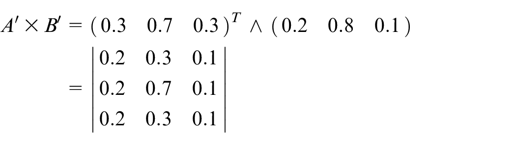
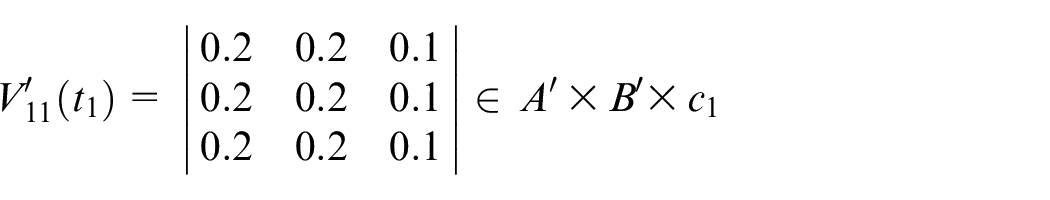
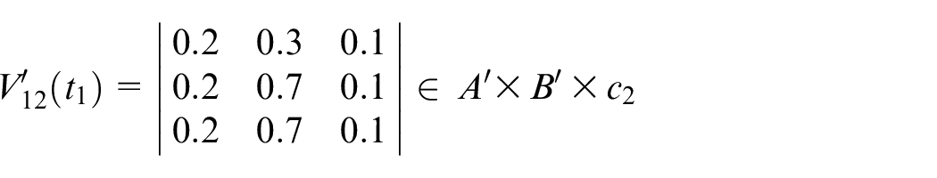
Step 2: Calculate fuzzy relational matrices V
V
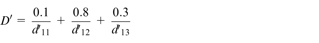
Step 3: Use the input data items to calculate the associated possibility difference denoted as
Step 4: If
If
|
Step 5: ∀ transition tj, fire the enabled transitions, perform the cylindrical extension and execute Zadeh’s max–min operation, that is, compute
Step 6: Return to Step 3 until no transition is available to be fired.
Step 7: Send the results to the core, transform them into the output place, and transfer the data sets to the supervisor place on the outer ring.
Step 8: Repeat the above steps until all input training data sets end.
The fuzzy production rules are shown as follows:
The predicate logic form is shown below.
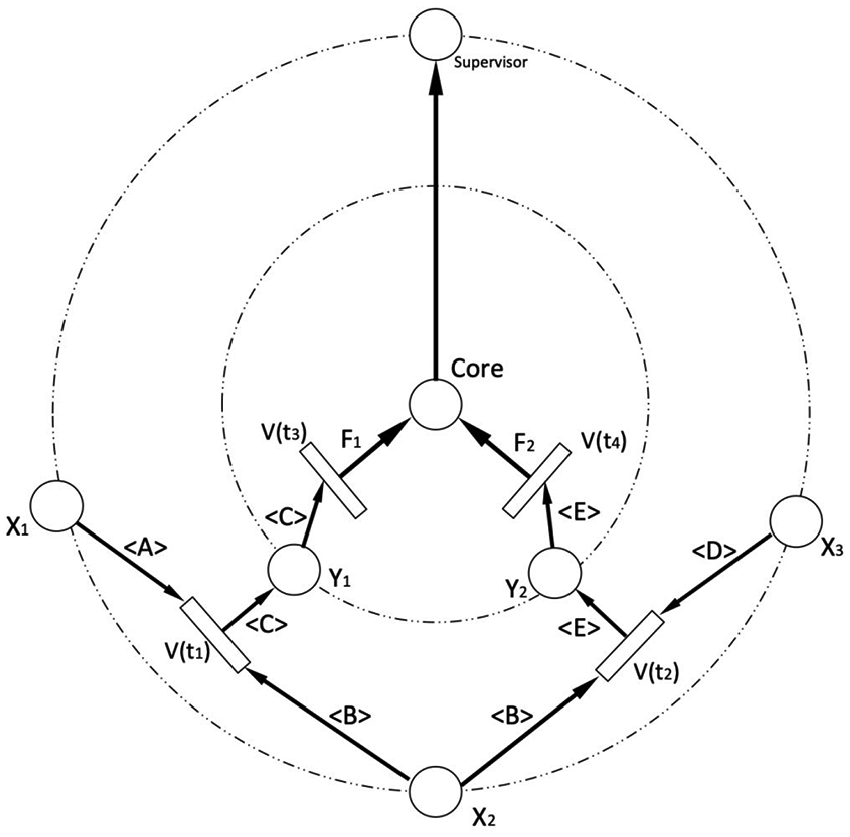
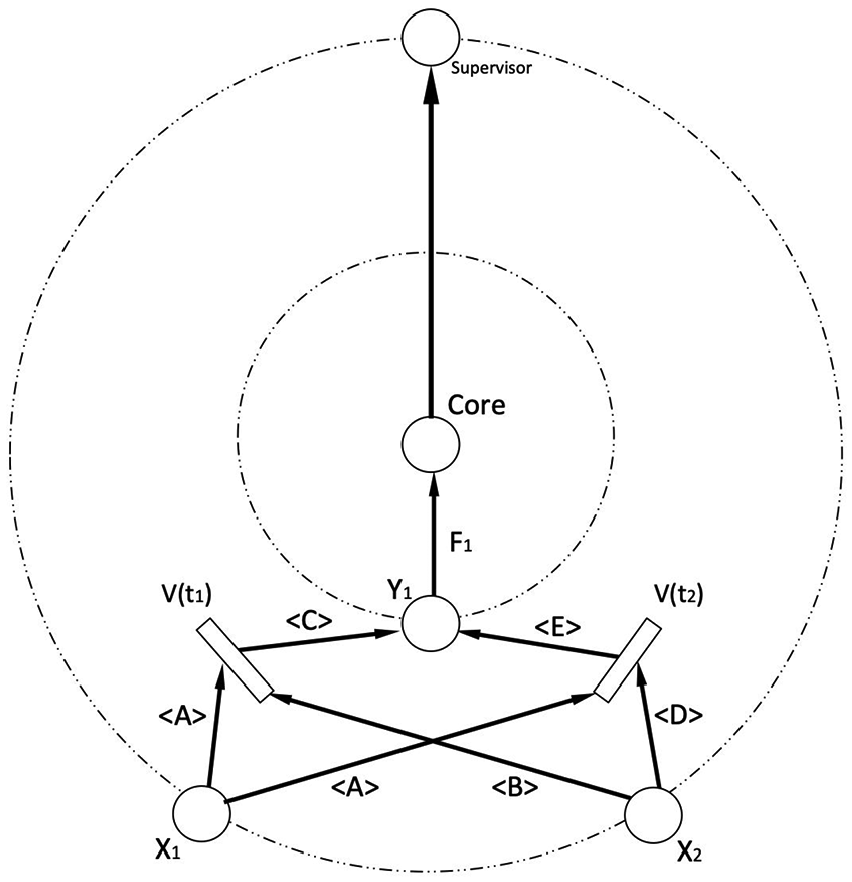
According to the predicate logic form shown above, we get Figure 1.
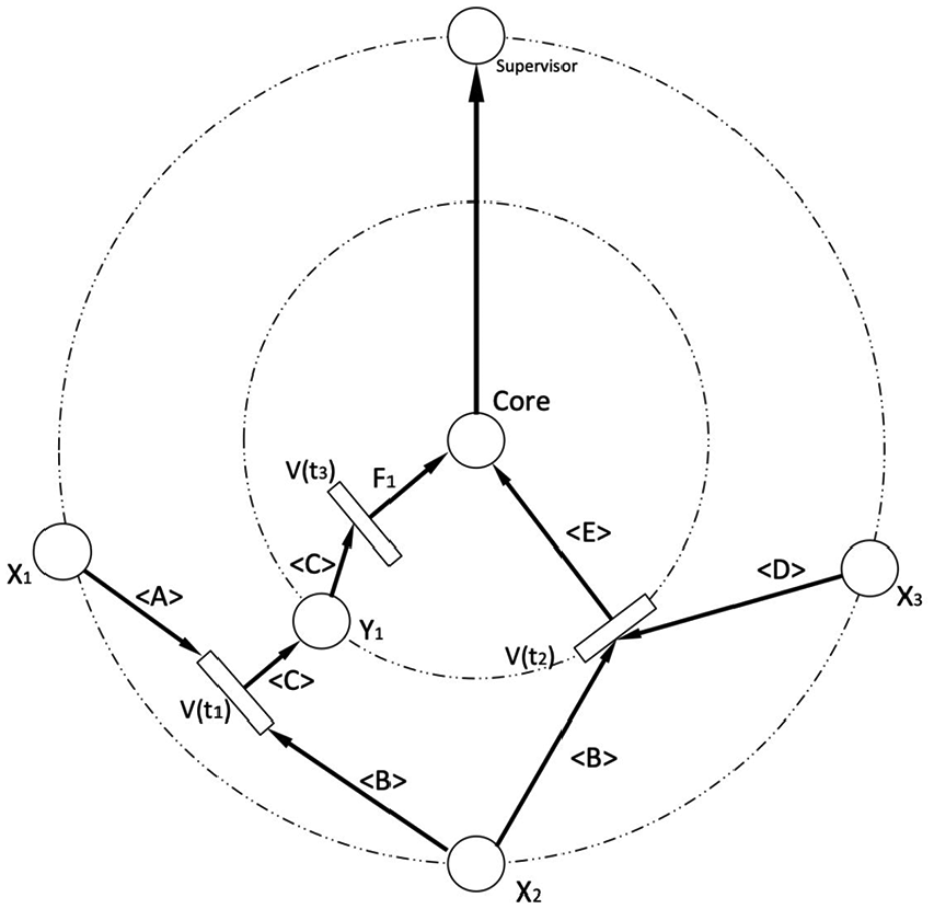
Unsupervised DPN for Example 1.
Numerical analysis
Step 1: Initialize
The initial marking is
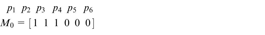
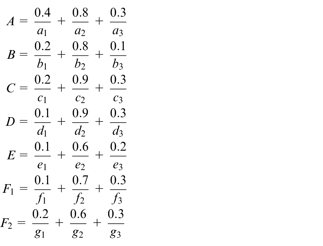
The data sets which are non-zero mean the token is available to fire its transition. Assume that the fuzzy sets are shown as follows:
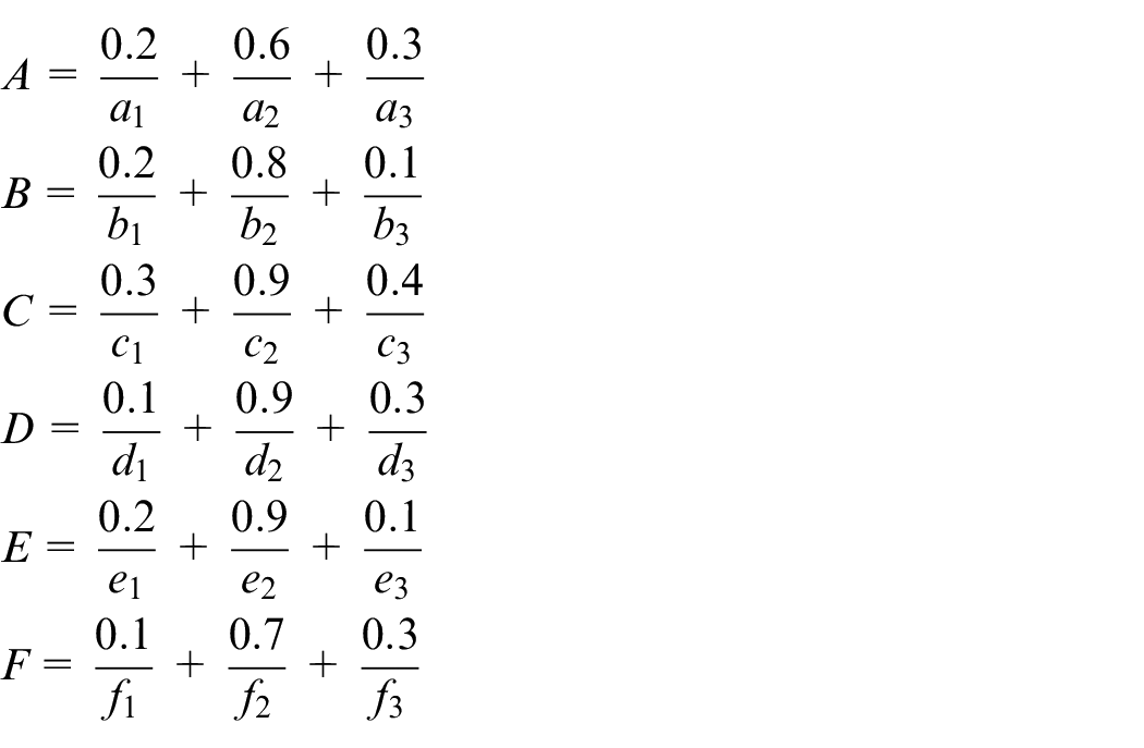
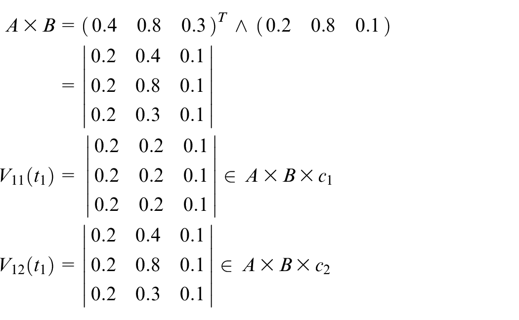
Step 2: Calculate the fuzzy relational matrices.
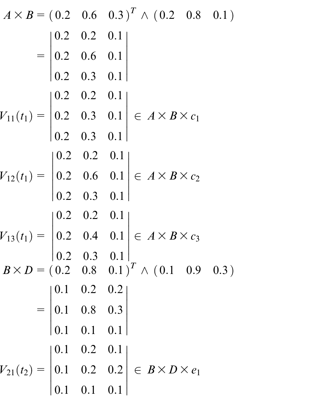
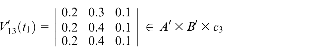
Steps 3–6: Assume that the first input data items are shown as follows:
Assume that the transition firing sequence is


Calculate


Assume


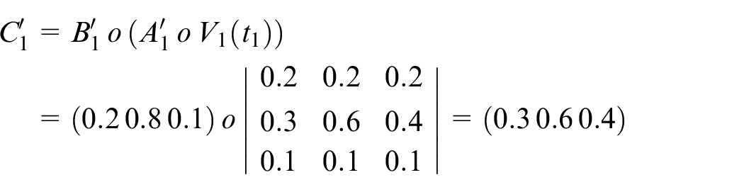


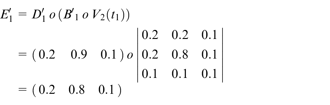
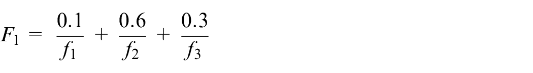
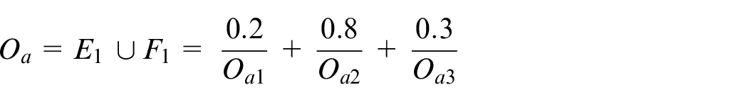
Step 7: Finally, the actual output is shown below
Step 8: Repeat the next iteration.
Supervised deep learning algorithm
The difference between unsupervised learning and supervised learning is that the core will perform supervised learning to confirm the convergence of the ring. If the situation is not done as expected, the core will feedback to the supervisor place on the ring to correct the attribution.
INPUT: Input place (IP) Mem
OUTPUT: Output place (OP) Mem
PROCEDURE:
Step 1: Initialize, check whether Mem
Step 2: Calculate the fuzzy relational matrices V
Step 3: Fire the enabled transitions, and execute Zadeh’s max–min operation.
Step 4: Return to Step 3 until no enabled transition is available.
Step 5: Send the results to the core and transform them into the output place. Transfer the data sets to the supervisor place on the outer ring.
Step 6: The desired output
Step 7: Recalculate the new fuzzy relational matrices
Step 8: Repeat the above steps until all input training data sets end.
The fuzzy production rules are shown as follows:
Thus, the predicate logic form is shown below.
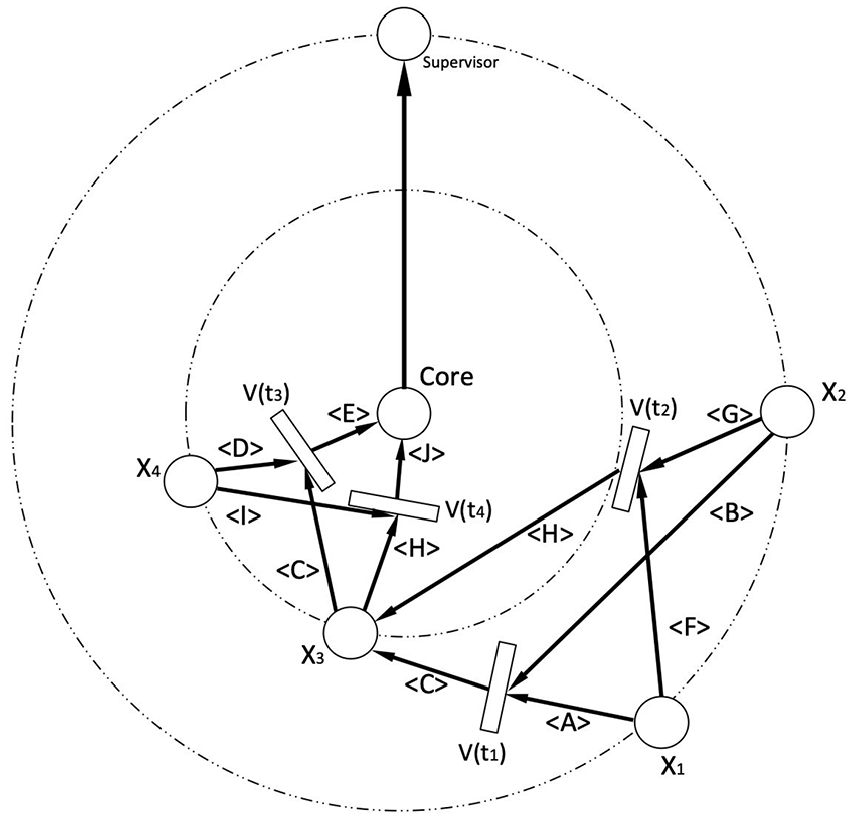
According to the predicate logic form shown above, we get Figure 2.
Supervised DPN for Example 2.
Numerical analysis
Step 1: Initialize
The initial marking is


The data sets which are nonzero mean the tokens are available to fire its transition.
Assume that the fuzzy sets are shown as follows:
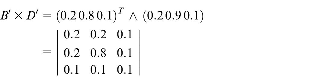
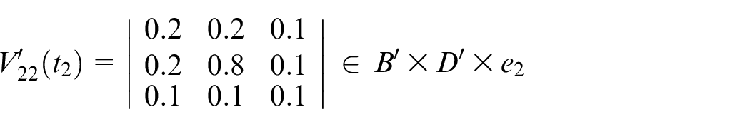
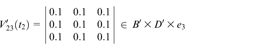
Step 2: Calculate the fuzzy relational matrices
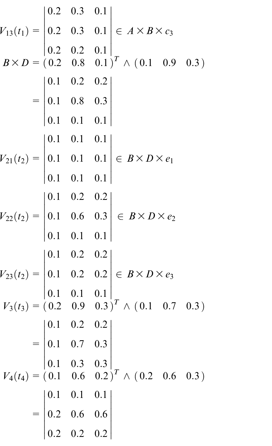
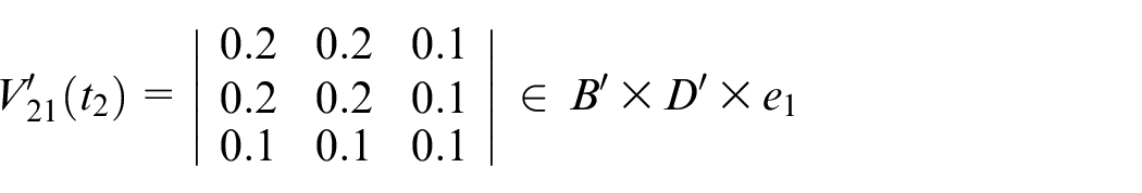
Steps 3–5: Assume that the first input data items are shown as follows

Assume that the transition firing sequence is
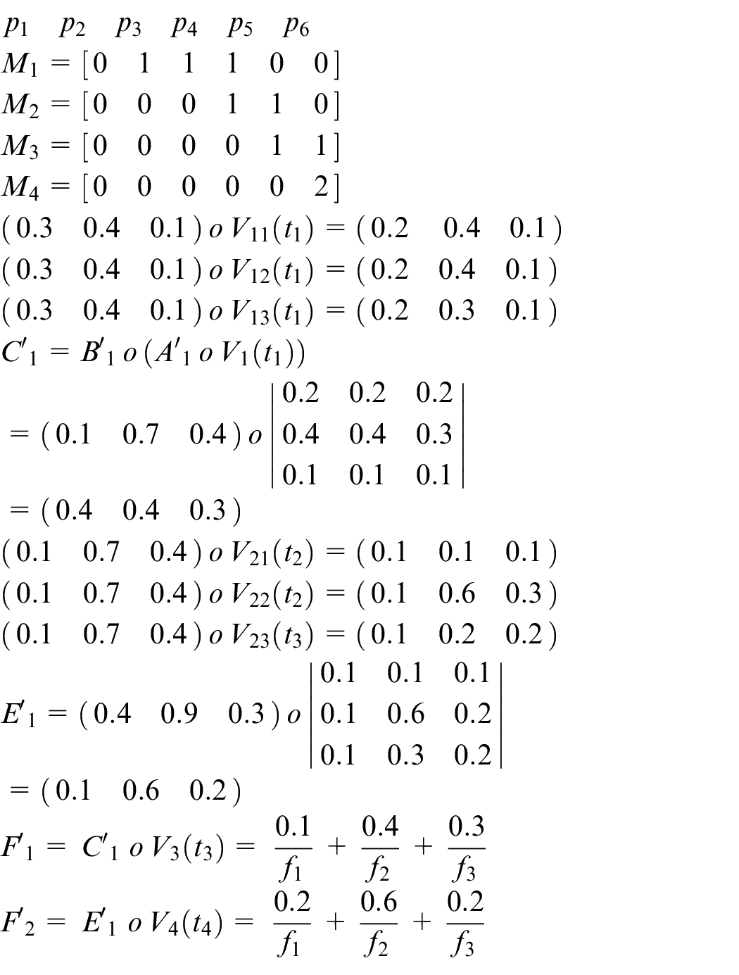
The actual output
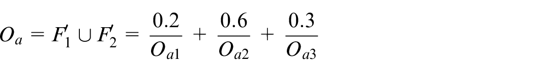
Step 6: The desired output
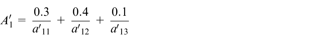
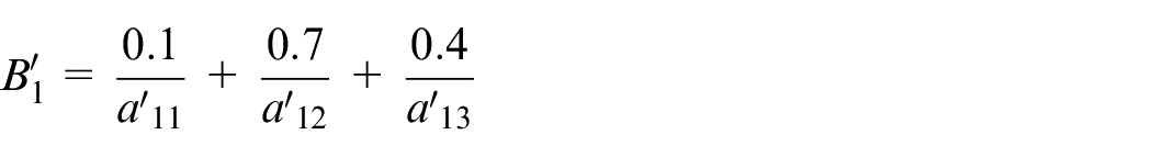
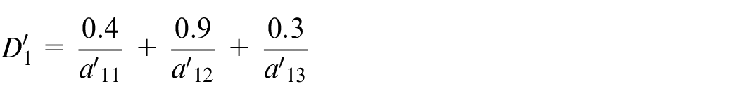
Assume that the desired output is
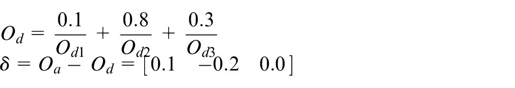
Step 7: Readjust all fuzzy sets and recalculate the fuzzy relational matrices as follows
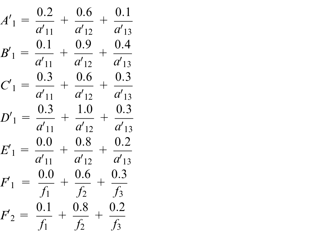
Step 8: Repeat the next iteration.
Main results
This section aims to analyze DPN. First, compare the structure of DNN with that of DPN. Then, by observing both structures, we illustrate examples to compare their characteristics.
Research tools
This is intended to compare DPN with DNN. The comparison action is taken by DPN, in which the environment uses the 2.2 GHz Intel Core i7 and the memory is 16 GB 1600 MHz DDR3. The DPN was implemented in C++.
The DNN is based on SONY’s Neural Network Cloud. It is an open source for system developers. Users can easily build the DNN models only by choosing what function they need without writing any program. 10
Benchmarks
The problem with fuzzy car is to figure out the car’s acceleration when it slides down from the top of U-shape track. The car has different numbers and different directions of acceleration in every moment. 16
The problem with Pole and Rotation is that when pulling the object, the stick on the object does not fall down. Under normal conditions, the stick will fall in the direction of acceleration, and the system needs to learn how to control the correct acceleration. It can move the main object so that the stick on the object does not fall down. 18
The t-Test is a benchmark used to compare the mean value of two data items and to check whether or not they are different. 3 The test can deal with the unknown variances and independent or small data items. In this sub-section, we only use the logic rules of t-Test to conduct our experiments. 19
Output-feedback fuzzy controller (OFFC) is a part of rotational/translational proof-mass actuator (RTAC). 4 OFFC acts as a nonlinear controller in RTAC. It can process the approximations without using exact mathematical quantities. In our experiments, we only use its processing logic rules to run the test of our structures.
The fuzzy production rules for fuzzy car logic are shown as follows:
IF the car
IF the car
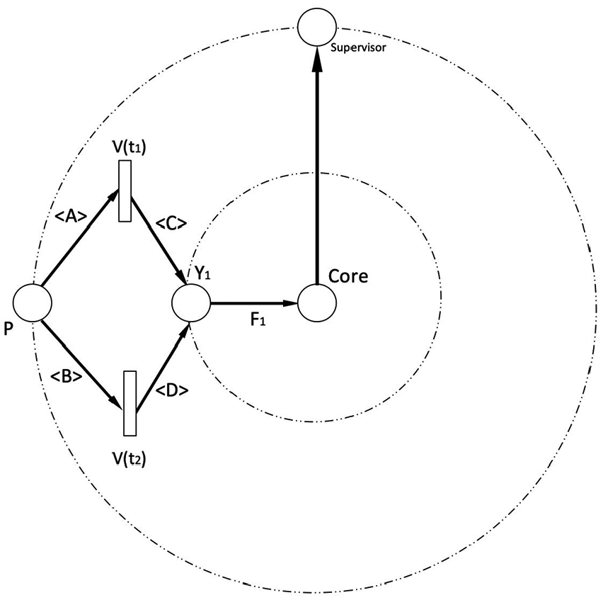
According to the fuzzy production rules shown above, we get Figure 3.
DPN of fuzzy car rules.
The fuzzy production rules for Pole and Rotation logic are shown as follows:
IF the pole direction
IF the car
IF the pole direction
IF the car
According to the fuzzy production rules shown above, we get Figure 4.
DPN of pole and rotation rules.
The fuzzy production rules for t-Test logic are shown as follows:
IF the number (P) is significant
IF the number (P) is not significant
According to the fuzzy production rules shown above, we get Figure 5.
DPN of t-Test rules.
The fuzzy production rules for OFFC logic are shown as follows:
IF the pointer (P) is positive
IF the pointer (P) is negative
IF the pointer (P) is positive
IF the pointer (P) is negative
According to the fuzzy production rules shown above, we get Figure 6.
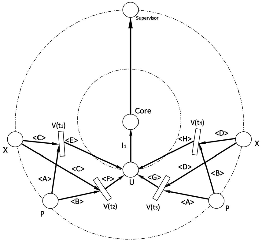
DPN of OFFC rules.
Experimental results
In this sub-section, the results of running four benchmarks are presented to evaluate the performance of the unsupervised learning DPN and the supervised learning DPN. Those experimental results regarding the unsupervised learning and the supervised learning algorithms are shown in Table 1.
Performance comparison between unsupervised learning and supervised learning.
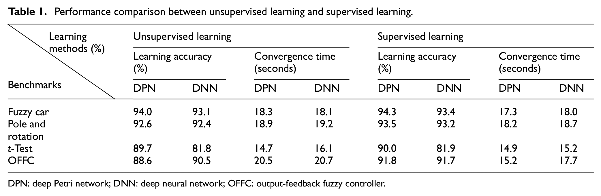
DPN: deep Petri network; DNN: deep neural network; OFFC: output-feedback fuzzy controller.
According to the experimental results in Table 1, we assemble those values in Figures 7 and 8.
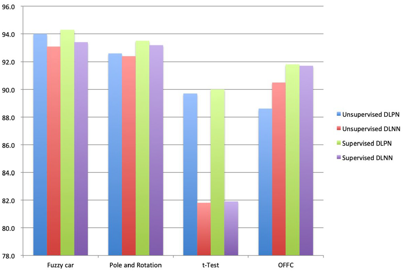
Learning accuracy of four structures.
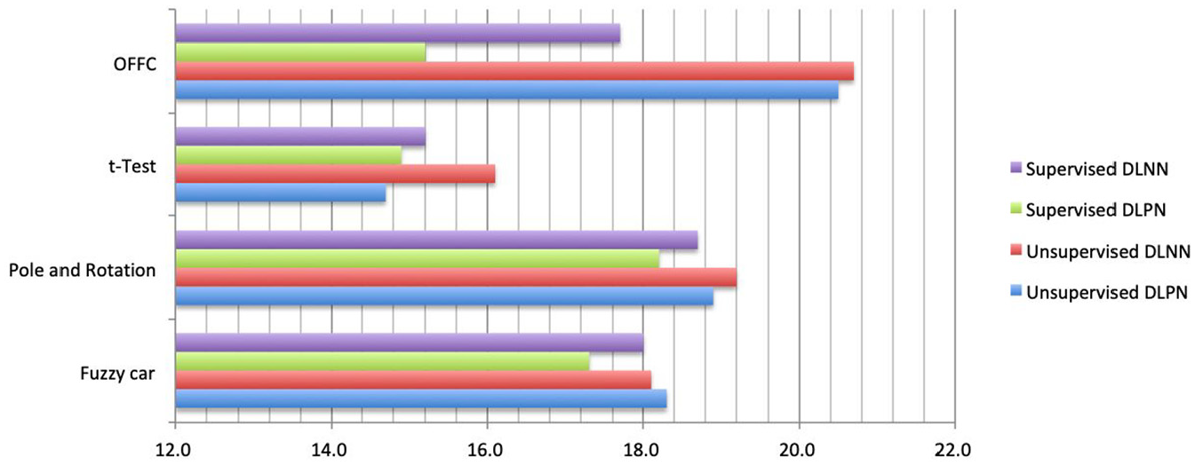
Convergence speed of four structures.
In summary, the experimental results in Figures 7 and 8 indicate that the learning accuracies of the unsupervised and the supervised learning DPN are larger than those of the unsupervised and the supervised learning DNN. In addition, the convergence times of the unsupervised and the supervised learning DPN are less than those of the unsupervised and the supervised learning DNN. Therefore, DPN is better than DNN for four types of benchmarks, and it is certain that DPN can better perform the unsupervised and the supervised deep learning than DNN.
Functional comparison
Based on the above experimental results, we compare the differences between two models of DPN and DNN, and obtain the main results shown in Table 2.
Functional comparisons.
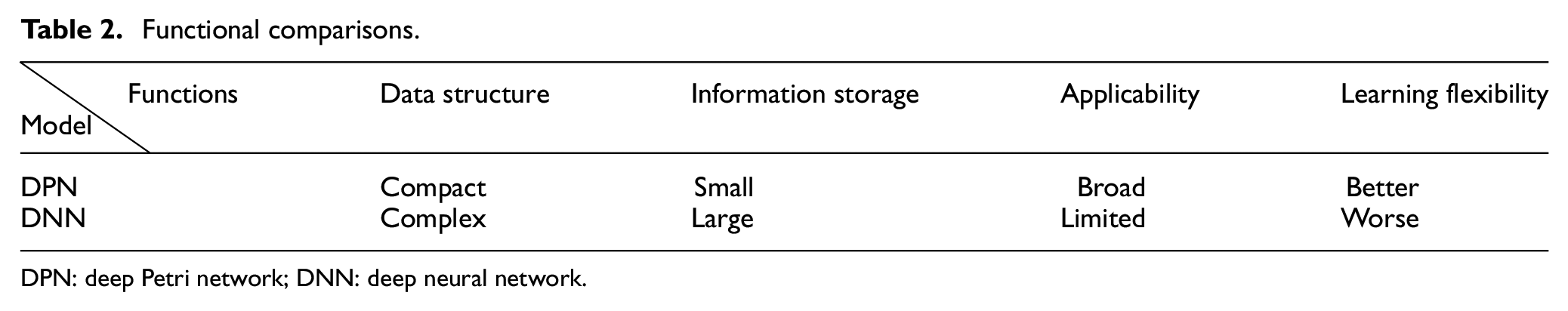
DPN: deep Petri network; DNN: deep neural network.
Conclusion
This article has successfully established the DPN model through Petri net theory, a new model for the unsupervised and supervised deep learning. The contributions of DPN are presented as follows:
The unfixed structure is different from the fixed fully connected structure of DNN. DPN is used to analyze the problem’s properties before establishing the structure of the problem.
Since each structure in DPN is designed for the problem itself, the nodes on the structure are only the necessary ones. So, the number of nodes in DPN is less than the ones in DNN for the same problem.
Because the number of nodes is smaller in DPN, the parameter adjustment is processed every time when the input data are finished, instead of making decision on the classification each time. Thus, the fewer number of nodes makes the overall convergence speed become faster.
However, the benchmarks used in this article are just uncomplicated logic. If one wants DPN to deal with other complicated types of data sets, such as image types or data streams, it will need to make more research efforts. It needs further research work regarding how to define an image or stream data types in fuzzy logic. If those types have complicated fuzzy relations, DPN will be further improved.
Footnotes
Acknowledgements
The authors are very grateful to the anonymous reviewers for their constructive comments which have improved the quality of this paper.
Declaration of conflicting interests
The author(s) declared no potential conflicts of interest with respect to the research, authorship, and/or publication of this article.
Funding
The author(s) disclosed receipt of the following financial support for the research, authorship, and/or publication of this article: This work was supported by the Ministry of Science and Technology, Taiwan, R.O.C., under grant MOST 107- 2221- E-845-001-MY3 and MOST 107-2221-E-845-002-MY3.