
Abstract
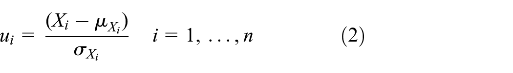
Quantiles are values of a function associated with specific probabilities. Two very specific quantiles, that is, ±3, are usually used for estimating probabilistic distribution of the function. Aiming at the engineering complex implicit function, the article provides an algorithm for calculating these values efficiently and rapidly. First, build kriging model with initial high-efficiency samples and the model is taken as the approximate initial analytical expression of the original function. Then, seek for the approximate most probable point with kriging model and performance measure approach. The most probable points found every time and their corresponding function responses are taken as new samples to reconstruct the built kriging model. After several times of reconstructing kriging model, the convergence value for the corresponding quantile can be obtained. Finally, the illustrative cases in this article demonstrate that the quantile-based method can provide accurate results with high efficiency and in this way, the quantile convergence value can be obtained by a few samples.
Introduction
In engineering applications, uncertainties exist in many problems. For example, machining errors in mechanism links lead to uncertainties; internal defects of material lead to uncertainties of physical parameters; and external environment leads to load uncertainties. Under the influence of these uncertain factors, many problems’ output also becomes uncertain. Considering its significance to engineering safety design, the uncertainty research has drawn wider attention and given rise to branches such as reliability research and robustness research.
The methods of uncertainty research include probabilistic approaches and non-probabilistic approaches. Non-probabilistic approaches include interval analysis,1,2 fuzzy theory, 3 possibility theory,4–6 convex theory, 7 and epistemic parameter uncertainty. 8 Relatively speaking, probabilistic approaches are more widely used. For example, Hamon et al. 9 conducted a sampling-based probabilistic security evaluation (PSE) of a high-power wind system. Sarsria and Azrar 10 studied the dynamic response of large structures under the influence of uncertainty factors with the perturbation method. Sepahvand et al. 11 proposed to use polynomial chaos expansion (PCE) to quantitatively analyze the uncertainties of stochastic systems. Zhao and Ono 12 put forward a universal program to analyze the reliability by the first-order, first-moment method and second-order, second-moment method. When Lee et al. 13 studied the reliability optimal design, they proposed an uncertainty calculation method of nonlinear and multidimensional systems, which is based on the most probable points (MPPs). Based on the dimension reduction method, Chowdhury and Rao 14 proposed a reliability calculation method of hybrid high-dimensional model under the influence of random factors. Wei et al. 15 proposed an active learning procedure combined with the multiple-response Gaussian process model and Monte Carlo simulation to efficiently and adaptively produce surrogate models for the failure surfaces of systems. Xiao et al. 16 proposed a new adaptive surrogate model–based efficient reliability method to compute structural reliability.
Generally speaking, probabilistic approaches are mainly composed of the following five categories: (1) simulation-based methods: Monte Carlo simulations and improved variance deduction method;17–19 (2) local expansion–based methods: Taylor series, 20 perturbation method, 21 and so on; (3) functional expansion–based methods: Neumann expansion, 22 PCE, 23 and so on; (4) MPP-based methods: first-order reliability method (FORM) 12 and second-order reliability method (SORM); 24 and (5) numerical integration–based methods: dimension reduction. 25 However, despite the big development of uncertainty researches, Methods (2)–(5) are only valid for certain problems under certain conditions. The above four methods are therefore not universal due to their limitations. Fortunately, Method (1) is universal and easy to use. Presently, there are two difficulties in calculating uncertainty for complex large-scale engineering problems: (1) the function is a black box and implicit; (2) the calculation requires business software such as finite element, resulting in a large amount of calculation. Under these two circumstances, only Method (1) is suitable. But the sample selection of Method (1) is random, resulting in slow convergence. In consequence, a considerable number of samples are needed to ensure that the results are accurate. Besides, it takes a long time to solve the large-scale and complicated problem every time. In case of conducting response calculation of a large number of samples, the complicated engineering problems will need to be solved repeatedly. Usually, the calculation cost is too high to carry out.
In view of the above, this article presents an efficient analytical method based on quantiles to determine the solutions at critical boundary probabilities. The method contains three ideas: first, evaluating the probability response range of the problem by means of the quantile; second, new samples are chosen close to the boundary probability; and third, reconstructing a surrogate model with new samples in order to make full use of the information provided by new samples and accelerate the surrogate model to approximate the real function and therefore make sure that the convergence of the response is accelerated. The article is organized as follows. Section “Concept of determining the uncertainty of function probability with quantile” introduces the concept of determining the probabilistic uncertainty of the function with quantile. Section “Fast method of calculating function quantile response value” presents a fast method of calculating the quantile response value of the function. Section “Case analysis” verifies the method proposed in this article through case analysis. Finally, section “Conclusion” summarizes the method proposed in this article.
Concept of determining the uncertainty of function probability with quantile
For any complex model, suppose its function to be

Input uncertain parameters lead to uncertain model output.
Figure 2 presents the probability distribution of function f.

Probability distribution of function f.
The quantile response value of the function can be calculated by the performance measure approach (PMA method) as shown in equation (1)

where
where
Obviously, equation (1) equals

Obviously, equation (3) equals
There are several advantages of using quantile to determine the function uncertainty. (1) Quantiles describe values of the function associated with defined probabilities. (2) Using the PMA method, the function response value at the quantile can be obtained with a small number of samples. Therefore, the quantile-based method to evaluate function probability distribution needs less calculation and achieves higher efficiency.
Fast method of calculating function quantile response value
Construction of high-efficient initial sample set
The high-dimensional model representation is a generic and quantitative tool for model assessment and analysis. Using this method, the high-dimensional relationship between the model input variable and the output variable can be obtained. 14 And the initial sample used in this method greatly improves its modeling accuracy. Therefore, by referring to the way of selecting initial samples in the above-mentioned high-dimensional model representation method, the initial samples selected of the article in the standard normal space are as follows

where
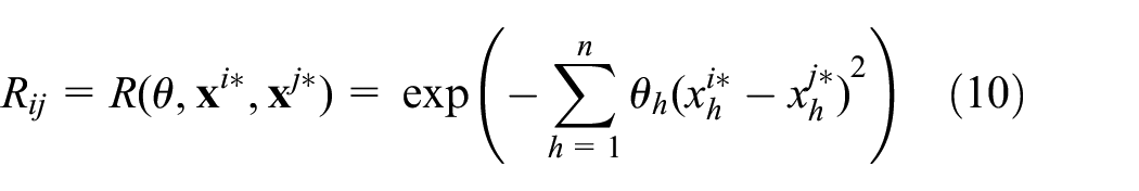
Kriging model
After the initial sample set

where

where
In equation (5),

where
In this article,

In equation (7),
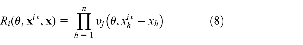
Fast calculation of function output for the quantile based on kriging modeling method
Build the initial kriging model with the initial set of samples
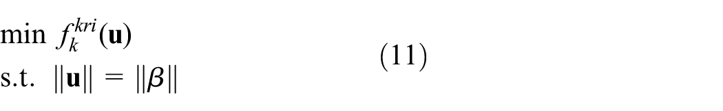
where k = 0, 1, 2, … indicates the times of model construction. By solving equation (11), the corresponding optimal solution
Add the optimal solution
Then compare, respectively, the convergence of the optimal solution


When equation (12) or (13) is satisfied, the calculation is stopped; otherwise, the above calculation is repeated. Finally, the resulting convergence value is the function response value of the corresponding quantile. Similarly, the convergence value of

Case analysis
Case 1
Example 1
Figure 3 shows a roof truss structure with a uniform load q and a node load P.22,27
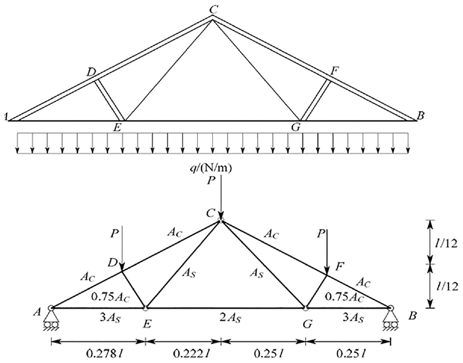
A truss structure.
The limit state function of the truss structure is

The above formula is called the limit state function which indicates that the downward deflection
Random variable parameter distribution in Case 1.

By substituting the average value in equation (15), the approximate mean value of the function response is 0.1766. Figures 4 and 5, respectively, represent the iteration calculation of the function response values of the left and right quantiles in Case 1. As for the left quantile

Left quantile function response value iteration calculation in Case 1.

Right quantile function response value iteration calculation in Case 1.
In order to verify the correctness of this method, the Monte Carlo method (hereinafter referred to as the MC method) is used to compute the structure, and then its mean value and standard deviation are calculated. Finally, the left and right quantiles are obtained according to equations (16) and (17), with the details shown in Tables 2 and 3. The MC calculation of the left and right quantiles in Cases 2 and 3 is the same as Case 1


Calculation results of function response value.

Comparison of results between MC method and the method in this article.
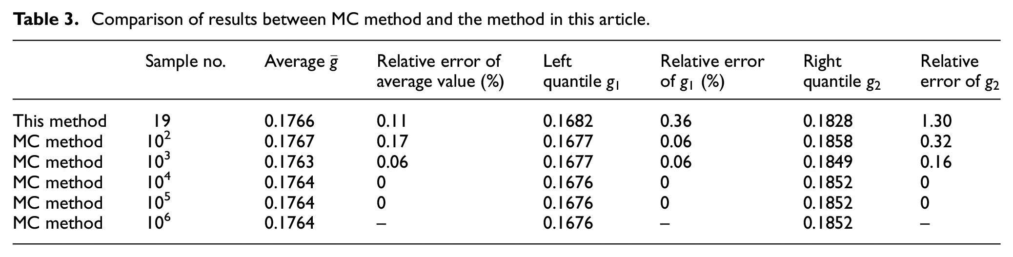
In Table 3, the calculated results of the MC method are used as the standard results and the relative errors are obtained by calculating the relative errors between the calculated results and the standard results. It can be found that the calculation results between the MC method and the presented method in this article are close to each other. In addition, the number of samples required for this method is much less than those of the MC method. Therefore, the calculation method used in this article is very efficient.
Case 2
Figure 6 shows a double-lap joint design of rubber-modified epoxy-based adhesive.
28
The design consists of aluminum outer adherent and an inner steel adherent. The completed bond is subjected to an axial load

A double-lap joint design of adhesive.
Distribution of the independent random variable parameters in Case 2.

The limit state function of the structure is the strength of the joint, that is, the maximum shear stress is less than the shear strength of the binder. When
The limit state function is the safety margin for strength requirement of the joint, which is defined by the difference between the lap-shear strength of adhesive and the maximum shear stress. The equation is obtained at

where

and

By taking the mean value of equation (18), the approximate mean value of the function response is 524.24. Figures 7 and 8, respectively, represent the iterative computation of the left and right quantile response of the function in Case 2. On the basis of 19 (2 × 9 + 1) initial samples, the left quantile

Left quantile function response value iteration calculation in Case 2.

Right quantile function response value iteration calculation in Case 2.
Calculation results of function response value.

The MC method is adopted for computing the structure and its computed results are used as the standard for comparing the results of the method used in this article. More detailed results are shown in Table 6. It can be found that the calculated results of this method are similar to those of the MC method, but the computational efficiency is much higher than that of the MC method.
Comparison of results between MC method and the method in this article.

Case 3
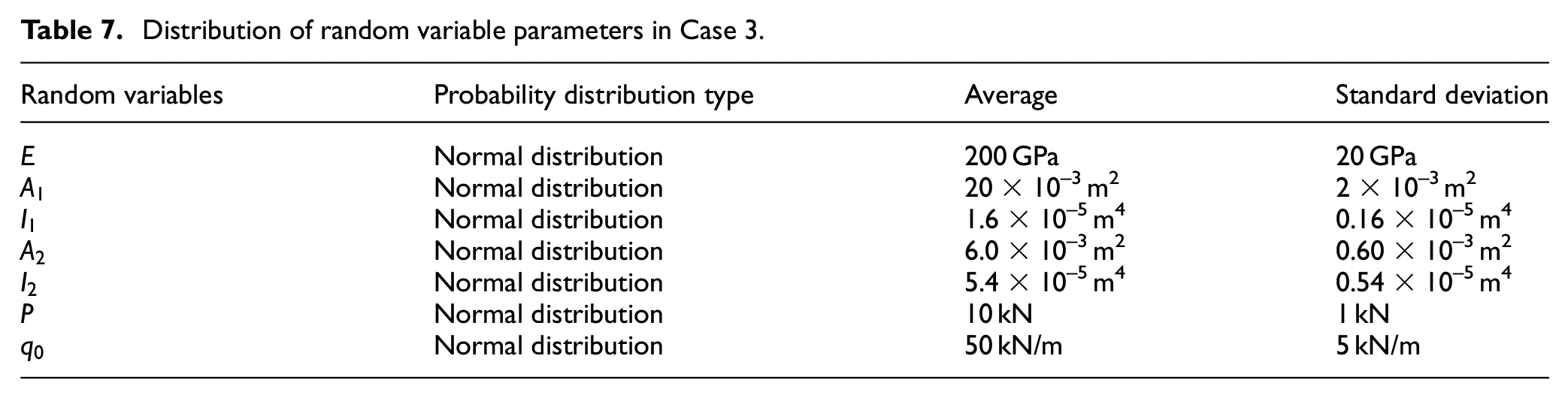
Figure 9 shows a structure consisting of three beams with two degrees of freedom. The details of the structural parameters are listed in Table 7.

Force figure of beam structure.
Distribution of random variable parameters in Case 3.
The structure requires that the maximum deformation under loads cannot exceed 0.2 m, as follows

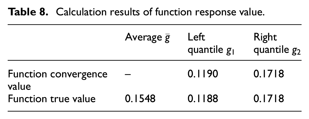
By substituting the average value in equation (19), the approximate mean value of the function response is 0.1548. Figures 10 and 11, respectively, represent the iterative computation of the left and right percentile response of the function in Case 3. On the basis of 15 (= 2 × 7 + 1) initial samples, they respectively converge to 0.1188 and 0.1718 after three and four times of iterations. The details of the results are shown in Table 8. A total number of 20 (= 15 + 3 + 2) calculated samples are needed to make sure the calculated results accurately converge to the real function response value for the corresponding quantile. Here, 15 represents the calculated number for initial samples; 3 and 2 represent the new generated samples when reconstructing the left quantile

Left quantile function response value iteration calculation in Case 3.
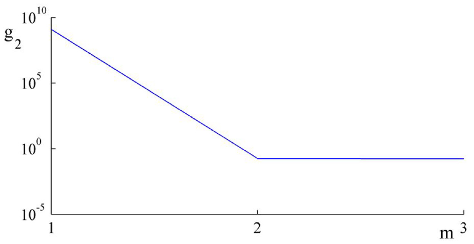
Right quantile function response value iteration calculation in Case 3.
Calculation results of function response value.
The structure is also computed by the MC method, and the corresponding results are used as the standard to compare the calculated results of the presented method. More detailed results are shown in Table 9. It can be found that the calculated results of this method are similar to those of the MC method, but the computational efficiency is much higher than those of the MC method.
Comparison of results between MC method and the method in this article.

Conclusion
In this article, a framework of calculating the function based on the quantile method is used to describe the stochastic uncertainty of the function. The main features of this method are as follows: (1) use the quantile conception to estimate the probability distribution of the function, namely, to determine the probability distribution range of the function based on the idea of the quantile. (2) Purposely select new samples, namely, according to certain strategy, that is, the PMA method, the new samples are chosen, thus overcoming the randomness in sampling and conducive to accelerate the calculation convergence. (3) Reconstruct the function, namely, by reconstructing the kriging model; it can fully absorb the information provided by the new sample and accelerate to approximate the real response value of the function at the quantile. The results of this article show that the method is accurate and reliable, the actual calculation time of the function is much lower than the MC method, and the calculation efficiency is extremely high.
The above-mentioned three features of this method have a strong reference. If this method is used, the computational efficiency of reliability and robustness optimization design can be greatly improved because these designs are involved with the uncertainty assessment of functions. Currently, the reliability and robustness optimization design of complex engineering still has problems, such as black boxes and excessive computation. In the future, related researches will be carried out to further expand the application of this method.
Footnotes
Acknowledgements
The authors thank Yuan Li and Zhongmou Ying for their helpful suggestions and careful modifications on English expressions.
Handling Editor: Michal Kuciej
Declaration of conflicting interests
The author(s) declared no potential conflicts of interest with respect to the research, authorship, and/or publication of this article.
Funding
The author(s) disclosed receipt of the following financial support for the research, authorship, and/or publication of this article: This study was supported by the National Natural Science Foundation of China (Grant Nos 51175194, 51405168, and 51305143), Promotion Program for Young and Middle-aged Teacher in Science and Technology Research of Huaqiao University (Grant No. ZQN-PY504), and Science and Technology Planning Project of Quanzhou (Grant No. 2017G045).