Sage Journals: Discover world-class research

Abstract

The characteristics of centrifugal pump in non-inertial stopping period have not been studied better by far. In this article, the variation characteristics of transient performance of a prototype pump are clarified experimentally in five non-inertial stopping scenarios and three typical steady-flow rates. The effects of stopping time on the transient performance during stopping periods are explored. Meanwhile, three non-dimensional parameters are employed to analyze the transient behavior as well. The results show that the shorter the stopping time is, the more obvious the decline delay phenomenon in rotational speed is at the end of non-inertial stopping. There is an obvious decline delay phenomenon in flow rate at the beginning of stopping. With increasing steady flow rate before stopping, both head and flow rate decline faster. Despite the difference in stopping time, the static pressures at the pump outlet demonstrate a similar variation feature, while those at the pump inlet exhibit different characteristics. The head damping is the fastest and then the shaft power and the flow rate are followed. The non-dimensional instantaneous flow rate, head, and shaft power have a similar evolution characteristic overall. The affinity law for centrifugal pumps can be adopted to predict the transient performance under the condition of large steady flow rate and in the superslow stopping scenario.

Keywords

Centrifugal pump non-inertial stopping stopping time affinity law damping characteristic

Introduction

Pump performance has been studied for hundreds of years, and the hydraulic efficiency and operating stability are becoming better and better. The transient-flow characteristics inside pumps and their performance also have become clearer and clearer.^1–4 However, in all these studies the steady working condition is aimed. But transient operating processes, such as sudden starting and stopping, can cause some relevant engineering problems; thus, the transient hydraulic performance of pumps has drawn more and more attention in recent years. Meanwhile, it is also found that the existing studies on transient performance of pumps are mainly focused on the abrupt starting process, while the studies on pump stopping characteristics are relatively less.

In some occasions, the pump stopping performance is vital to the operating reliability of related devices. For example, the nuclear reactor coolant pump would be in a state of coastdown when it loses driving power. Under the state of coastdown, the hydraulic performance of the nuclear reactor coolant pump is directly related to the safety of the nuclear reactor. Therefore, with increasing engineering demand day by day, it becomes more and more necessary to fully understand the transient performance of pumps during stopping periods, especially in some special occasions.

Tsukamoto et al.⁵ clarified the transient characteristics of a low-specific-speed centrifugal pump during stopping periods through performance testing and theoretical prediction. It was shown that the impulsive pressure and the lag in circulation formation around impeller blades are the main reasons for the difference between transient and quasi-steady characteristics.

Lefebvre and Barker⁶ measured the transient performance of a mixed-flow pump during startup and stopping periods. The results showed that the quasi-steady hypothesis was not suitable to predict the pump transient performance. Thanapandi and Prasad,^7,8 experimentally investigated the transient behavior of a volute pump during stopping periods and originally used the method of characteristics to analyze the transient performances quantitatively. It was found that each performance parameter’s decrement was not synchronized, wherein the decline in both flow rate and head was more rapid than that of rotational speed.

Tanaka and Tsukamoto⁹ found that the unsteady pressure and flow rate were related to the cavitation behavior during rapid starting and stopping periods. The oscillation cavitation or water column separation during transient periods was the main reason for the fluctuation in pressure and flow rate.

Rong et al.,¹⁰ for the first time, adopted the bond graph method to theoretically calculate the transient performance of a centrifugal pump during starting and stopping periods. The results agreed well with the experimental measurements, and this method could be used for other transient processes.

Liu et al. built a closed-loop system including pump model and tank and employed the dynamic mesh method and volume of fluid (VOF) mixture model to solve the unsteady flow in the whole system. Through numerical simulation, the transient performance and internal unsteady flow field in the pump model were obtained during stopping periods.¹¹ It was found that at the beginning of stopping process, there was a jump phenomenon in static pressure at the pump inlet. The predicted vortex in the impeller was thought to be the main reason for the deviation of the quasi-steady hypothesis from the actual performance in the transient stopping process prediction.

Wu et al.¹² studied the influence of rotor inertia magnitude and braking time on transient hydraulic performance of a radial pump during stopping periods by installing a flywheel with different mass. It was found that the kinetic energy stored in the wheel could drive the impeller in rotation for longer time after the motor was shutdown. Meanwhile, the kinetic energy stored in the pipe-loop allowed the flow not to stop immediately when the impeller no longer rotated.

According to the energy conservation equation of one-dimensional pipe system, Gao et al.¹³ put forward a model to predict the transient performance of nuclear reactor coolant pumps during flow coastdown period. The flow inertia stored in pipe system was the main reason for flow delay. In the case of large moment of inertia, the moment of inertia determined flow delay phenomenon.

Chen et al.¹⁴ measured the transient hydrodynamic performance of a mixed-flow pump at different rotational speeds. The polynomial equations based on quasi-steady hypothesis could be used to describe the actual performance curves. Wang et al.¹⁵ studied the effect of different running down models on hydraulic performance of a nuclear reactor coolant pump during stopping period.

In our previous works,^16,17 the transient characteristics of a centrifugal pump with a semi-open impeller were measured and explained.

As it can be seen from the existing results that a running down process, namely, the driving motor no longer provides a driving torque, is mainly addressed when the stopping characteristics of a pump are clarified.

In our latest work,¹⁸ the stopping characteristics of a pump delivering different media with various viscosities were numerically calculated under a few decline profiles of rotating speed. In that study, a typical non-inertial stopping process was distinguished from the running down process. To date, there is no experimental work on non-inertial stopping process for centrifugal pumps.

In this regard, the decline characteristics of pump’s rotational speed were controlled during stopping period using a frequency converter, and various on-inertial stopping processes were realized experimentally. The transient hydraulic performance of a shelf-priming centrifugal pump was measured during those processes.

Experimental pump, test rig, and method

Tested pump

The experimental pump is an overhung self-priming centrifugal pump of type DKS18-40-3, which belongs to a kind of centrifugal pump, as shown in Figure 1. The pump specifications at the design point include the rotational speed n_D = 2900 r/min, flow rate Q_D = 10 m³/h, head H_D = 35 m, pump inlet diameter D_j = 60 mm, pump outlet diameter D_o = 60 mm, impeller inlet diameter D₁ = 40 mm, impeller diameter D₂ = 166 mm, blade inlet width b₁ = 8 mm, outlet width b₂ = 8 mm, blade inlet angle β₁ = 40°, outlet angle β₂ = 20°, and the inlet width of volute D₃ = 22 mm. The gas–liquid separation chamber is with the depth, width, and height dimensions of 85 mm × 200 mm × 170 mm, respectively (measured from the impeller center), and the radius of the bottom semicircle of the chamber is 100 mm.

Figure 1.

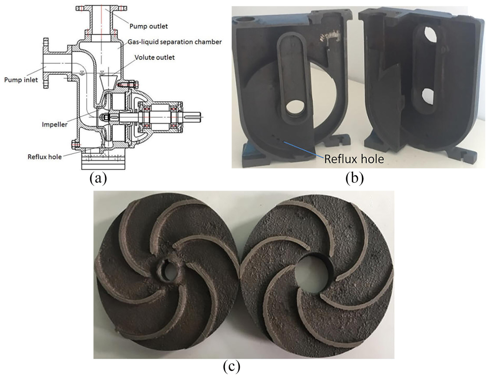
(a) Experimental pump axial cross-section drawing, (b) dissected gas-separation chamber, and (c) dissected impeller.

Test rig

The test rig used to measure the non-inertial stopping performance of the self-priming centrifugal pump as shown in Figure 2. The driving motor is a three-phase AC motor of 4.0 kW with a frequency converter. The frequency converter of type MICROMASTER 440 made by SIEMENS in Germany is used to control the magnitude of steady rotational speed before stopping, the decline time, and the decline characteristics of rotating speed. A torque detector of type JC0 with the range of 0–20 N m is adopted to measure the instantaneous rotational speed and shaft power with the total uncertainty of ±0.65% and an accuracy rating of 0.2 in them. An electromagnetic flowmeter of type OPTIFLUX 2100C with the range of 0–30 m³/h is utilized to measure the instantaneous flow rate with an uncertainty of ±0.5% and an accuracy rating of 0.5. Two pressure transmitters of type WIKA S-10 are used to monitor the instantaneous pressures at the pump inlet and outlet with the ranges of −0.1 to 0.1 MPa and 0–1.6 MPa, respectively, and with an uncertainty of ±0.75%. The measurement accuracy is less than 0.25% for both transmitters. The output signals of the measured parameters are all 4–20 mA current signals, which are acquired and processed by PCI8361BN card. The diameters of inlet and outlet pipes are 60 and 50 mm, respectively, and its lengths are 3 and 5 m, respectively. The material is steel pipe. The suction valve and discharge valve are both ball valves, and its maximum diameters are 60 and 50 mm, which are the same as pipes. The distance between suction valve and pump inlet is 2.5 m, while another distance between discharge valve and pump outlet is 4.5 m. In this article, the fluid tested is tap water at 20°C, its density is ρ=998.2kg/m³, and the dynamic viscosity is μ=1.0069×10⁻³ Pa s.

Figure 2.

(a) Test rig 3D model and (b) tested centrifugal pump unit.

Experimental method and scheme

The operational parameters of the frequency converter were used to control the decline time and profile of electric current supplied to the electric motor. As a result, the decline time and rule of rotational speed of the pump shaft were obtained.

In this article, the expected initial steady pump rotational speeds are 2900 r/min before stopping. Due to instantaneous voltage fluctuation in testing, the actual initial rotational speed fluctuated slightly around 2900 r/min. The expected durations of rotational speed in deceleration were specified to be 1.0, 3.0, 5.0, 7.0, and 9.0 s, respectively, which are called as five stopping scenarios: ultrafast, rapid, moderate, slow, and superslow stopping states. In this article, a linear decline profile was stipulated to control the electric current in the frequency converter with time; therefore, the rotational speed of the pump should decrease linearly with time theoretically. In other words, the decline of rotational speed is controlled, that is, the pump will experience a non-inertial stopping.

In each non-inertial stopping scenario, the initial steady pump flow rate can be altered by changing the discharge valve opening before stopping. In the experiment, three expected initial steady flow rates are Q₀ = 7.0, 10.0, and 13 m³/h, respectively, defining three pump working points, namely part-load, design, and over-load points. Considering three non-inertial stopping scenarios, there are 15 experimental cases and are summarized in Table 1.

Table 1.

Experimental case in stopping performance measurement.

Stopping scenario	Ultrafast	Rapid	Moderate	Slow	Superslow
Expected steady rotational speed, n (r/min)	2900	2900	2900	2900	2900
Expected duration of rotational speed in deceleration, t_e (s)	1.0	3.0	5.0	7.0	9.0
Linear deceleration of rotational speed, (rad/s²)	303.69	101.23	60.74	43.38	33.74
Expected initial steady flow rate, Q₀ (m³/h)	7 (part-load), 10 (design), and 13 (over-load)

The testing steps of the transient performance are as the following during non-inertial stopping periods. The entire circulation pipe line is filled with water before testing and making sure that the free surface in the tank is always higher than the elevation level of the tested pump and pipeline system. The suction valve is always completely opened; therefore, no cavitation appears. Then the electric currents of 50 Hz frequency are set in the frequency converter, where 50 Hz is for 2900 r/min steady rotational speed under the condition of 220 V. Then, the pump unit is started, and after the final steady rotational speed is reached, the discharge valve opening is changed to get the expected flow rate in Table 1. Once the pump speed is steady, then the pump is stopped, wherein the discharge valve opening is kept unchanged. It should be noted that before non-inertial stoppings, the decline time and decline rule of the electric currents need to be set in the frequency converter, and then carrying out stopping tests. During the transient process, the sensors will record the time history of every performance variable. As such, the transient performance curves can be obtained.

Results

Rotational speed

In the non-inertial stopping process, the instantaneous rotational speeds tested through torque detector are shown in Figure 3. At the part-load, design, and over-load points, the tested average steady rotational speeds before non-inertial stoppings are 2938, 2924, and 2906 r/min, respectively. In other words, the steady rotational speed should slightly decline with the increase of steady flow rate. This is due to the fact that the shaft power can be increased with increasing steady flow rate, making the motor load high and the final steady rotational speeds low.

Figure 3.

The instantaneous rotational speeds: (a) Q₀ = 7 m³/h, (b) Q₀ = 10 m³/h, and (c) Q₀ = 13 m³/h.

Experimental results show that the rotational speeds basically decline in accordance with the linear rule overall. Meanwhile, it is found that in the ultrafast and rapid two states, the rotational speeds deviate from the linear rule at the end of non-inertial stopping. There is a delay phenomenon in rotational speed, especially in ultrafast stopping state. Obviously, the shorter the stopping time is, the more significant the rotational speed deviation is due to an excessive deceleration in the speed.

In the case of ultrafast stopping, the length of time with a linear profile is about 1.10 s under three steady working conditions, the corresponding rotational speed is around 130 r/min.

In the part-load case of 7 m³/h, the times required for impeller stopping rotation at five stopping states are 1.547, 3.328, 5.188, 7.187, and 9.141 s, respectively. At the design point of 10 m³/h, the times required for the stop are 1.547, 3.296, 5.219, 7.172, and 9.172 s, respectively. Similarly, in the over-load case of 13m³/h, the times are 1.531, 3.297, 5.187, 7.172, and 9.125 s, respectively.

Obviously, in any non-inertial stopping processes, the final required times for stopping completely are longer than the timed assigned in advance. Since the decrease in rotational speeds is actively controlled through the frequency converter here, the deviation in the time between measurement and setting is not very obvious.

An additional parameter called characteristic damping time (t_n) is introduced to reveal the time effect of variable performance parameter during non-inertial stopping periods. The characteristic time is defined as the time length at which the pump speed has been declined by 63.2% of the initial steady speed.⁵

For the rotational speed, the ratio (λ_n) of the damping characteristics time (t_n) to the whole actual stopping time (T_n) is obviously different from one scenario to another. In the ultrafast case of 1.0 s, λ_n is basically around 0.47. In the rapid case of 3.0 s, λ_n is around 0.60. However, in the other stopping cases, λ_n is around 0.62. Thus, at the early stage of non-inertial stopping, the shorter the stopping time, the faster the decline of rotational speed.

Flow rate

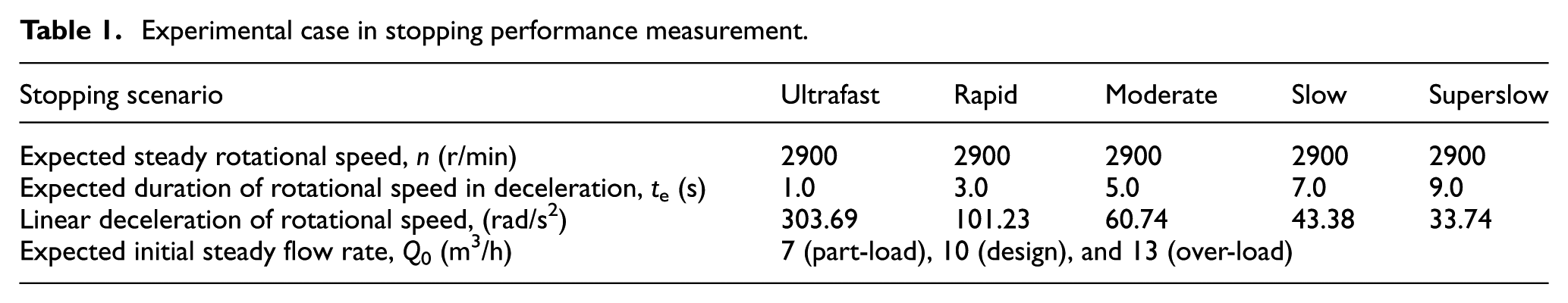
During non-inertial stopping periods, the instantaneous flow rates measured with the electromagnetic flowmeter are shown in Figure 4. Compared with the linear decline rule in rotational speeds, the decline rule in flow rates is not strictly linear. Specially, the decline characteristics of flow rate are markedly different from one stopping state to another or across the time span during one stopping state. For example, at the beginning of non-inertial stopping, the flow rates do not immediately decrease; instead, there is a significant delay in decline, namely hysteresis. This phenomenon was also found in the inertial stopping process.¹² In three steady flow rate cases, a flow rate just begins to decrease at about 1.0 s. Furthermore, with the extension of stopping time assigned, the flow rate starts to decrease at an increasingly delayed time.

Figure 4.

The instantaneous flow rates: (a) Q₀ = 7 m³/h, (b) Q₀ = 10 m³/h, and (c) Q₀ = 13 m³/h.

In the ultrafast and rapid non-inertial stopping cases, the flow rates decline almost linearly, except at the early and late stages. In three non-inertial stopping cases, such as moderate, slow, and superslow, the flow rates basically decline linearly at the middle and later stages. No matter what the stopping state is, there is a hysteresis in the flow rate decline to a certain degree at the end of non-inertial stopping.

At the part-load point of 7 m³/h, the times required for flow to completely stop are 4.063, 8.656, 12.907, 15.718, and 20.032 s, respectively, for five non-inertial stopping scenarios. At the design point of 10 m³/h, the times for flow to completely stop are 4.797, 8.531, 12.250, 16.234, and 20.172 s, respectively, for five non-inertial stopping scenarios. Similarly, at the over-load point of 13 m³/h, the times are 5.593, 8.938, 12.937, 16.750, 20.531 s, respectively, for five non-inertial stopping scenarios.

Interestingly, the times for flow to completely stop increases gradually with increasing steady flow rate before stoppings in ultrafast, slow, and superslow non-inertial stopping cases. In the other cases, however, this effect does not exist.

Like the definition of damping characteristics time of rotational speed, the flow rate damping characteristic parameter (λ_Q) is defined as the ratio of the flow rate damping characteristic time (t_Q) to the whole flow stopping time (T_Q). The flow rate damping characteristic time (t_Q) is also defined as the time length at which the flow rate has been declined by 63.2% of the initial steady value. At the part-load point of 7 m³/h, the ratios λ_Q of five non-inertial stopping scenarios are 0.659, 0.664, 0.706, 0.719, and 0.709, respectively. At the design point of 10 m³/h, the ratios are 0.557, 0.626, 0.648, 0.692, and 0.663, respectively. At the over-load point of 13 m³/h, the ratios are 0.486, 0.613, 0.627, 0.660, and 0.645, respectively. For all the scenarios, the ratios exhibit a gradual decrease trend with increasing steady flow rate before stopping. This suggests that the decline of flow rate is more dominant in the first half of non-inertial stopping than in the second half.

Meanwhile, except the superslow case of 9.0 s, the ratios gradually increase with extension of stopping time, manifesting that the decline of flow rate is slowed. This is because with the extension of stopping time, the speed deceleration becomes smaller and is concomitant with a slowly declined flow rate.

Static pressure at inlet

The instantaneous static pressures at the pump inlet monitored with the pressure sensor are shown in Figure 5. The characteristics of static pressure variation vary clearly from one non-inertial stopping scenario to another. At the part-load, design, and over-load points, the initial static pressures at the inlet are 5.7, 3.5, and −1.4 kPa, respectively, showing a tendency of gradual decrease. This is because with increasing steady flow rate before stopping, the fluid velocity at the inlet is increased, which makes a decreased static pressure.

Figure 5.

The instantaneous static pressures at the pump inlet: (a) Q₀ = 7 m³/h, (b) Q₀ = 10 m³/h, and (c) Q₀ = 13 m³/h.

For the ultrafast scenario of 1.0 s, the static pressures exhibit an oscillating pattern initially and then attain steady values. At three working points, at first, the maximum static pressures have achieved 14.36, 13.70, and 10.58 kPa values, respectively, suggesting gradually decreasing tendency. Then the pressures experience the local minimums of 8.52, 9.02, and 8.08 kPa, respectively. Once again, the pressures begin to increase to achieve the local maximums of 13.42, 12.78, and 13.48 kPa. Subsequently, the static pressures begin to decrease again until the steady value of 9.0 kPa.

In the rapid, moderate, slow, and superslow scenarios, the shape of the static pressure curves is simpler, namely they first increase and then decrease. With the extension of the stopping time, the curves become flat gradually. The reason for rising pressure is that with decreasing flow rate during non-inertial stopping periods, the velocity at the inlet is lowered, which makes the static pressure increase. As a result, the maximum static pressure caused by the flow inertia of the liquid in the pipe system exceeds the static pressure of the static liquid after stopping. However, the liquid in the pipe system gradually stops flowing, that is, the flow inertia gradually diminishes, which makes the static pressure gradually recover to decrease until a steady value. Under the conditions of three steady flow rates (part-load, design, and over-load) and four stopping scenarios (rapid, moderate, slow, and superslow), the final steady static pressures or the pressure of the static liquid is 9.0 kPa.

For the rapid stopping scenario of 3.0 s, the achieved maximum static pressures are 10.28, 10.62, and 10.32 kPa at three steady-flow rates, and the corresponding times are 6.297, 6.031, and 6.297 s, respectively. The times required for the static pressure to decrease to the steady value of 9.0 kPa are 8.047, 8.531, and 8.204 s, respectively.

For the moderate stopping case of 5.0 s, the achieved maximum static pressures are 9.74, 9.96, and 10.06 kPa at three steady flow rates, and the corresponding times are 10.485, 11.031, and 10.843 s, respectively. The times for decreasing to 9.0 kPa are 11.641, 11.703, and 12.031 s, respectively.

For the slow stopping case of 7.0 s, the achieved maximum static pressures are 10.12, 10.16, and 10.28 kPa at three steady flow rates, and the corresponding times are 14.25, 14.328, and 14.688 s, respectively. The times for decreasing to 9.0 kPa are 16.437, 16.531, and 16.485 s, respectively.

For the superslow stopping case of 9.0 s, the achieved maximum static pressures are 9.76, 9.88, and 9.96 kPa at three steady flow rates, and the corresponding times are 18.485, 18.844, and 18.921 s, respectively. The times for decreasing to 9.0 kPa are 20.063, 20.172, and 20.343 s, respectively.

It is found that with extension of the stopping time, the required times for achieving maximum and steady pressures are gradually prolonged. However, the individual maximums show little variation, that is, around 10.0 kPa. This is because of the fact that the flow inertia of the liquid in the pipe system plays a main role in determining the maximum static pressure.

Static pressure at outlet

The measured instantaneous static pressures at the pump outlet during non-inertial stopping periods are shown in Figure 6. It can be seen that the evolution characteristics of static pressure curves at the outlet have a similarity for five stopping scenarios.

Figure 6.

The instantaneous static pressures at the pump outlet: (a) Q₀ = 7 m³/h, (b) Q₀ = 10 m³/h, and (c) Q₀ = 13 m³/h.

For a steady flow rate, the static pressure curves follow a parabolic rule approximately. As we know, the static pressure at the outlet is approximately proportional to the squared rotational speed according to the affinity law for centrifugal pumps. In this article, the rotational speeds approximately decrease in accordance with a linear rule, so the static pressures at the outlet should exhibit an approximate parabolic profile.

With extension of stopping time, the parabolic rule is demonstrated even more clearly. This indicates that with extension of stopping time, the affinity law for the steady working condition of centrifugal pump is more suitable to the non-inertial stopping process except the ultrafast scenario.

At the part-load, design, and over-load points, the final static pressures at the outlet are all about 9.50 kPa in five stopping scenarios, which is slightly higher than the steady static pressure of 9.0 kPa at the inlet. The difference of liquid static height between the inlet and the outlet is responsible for the static pressure difference across the inlet and outlet in the steady state.

At the part-load point of 7 m³/h, the times required for the static pressures at the outlet to decrease to the final steady value of 9.50 kPa are 3.734, 7.015, 10.907, 15.140, and 19.063 s, respectively. At the design point of 10 m³/h, the times required for the static pressures to decrease to 9.50 kPa are 4.031, 7.718, 11.516, 15.891, and 19.390 s, respectively. At the over-load point of 13 m³/h, the times are 4.390, 8.141, 11.937, 16.113, and 19.531 s, respectively. This suggests that with increasing steady flow rate, the time required for the static pressure at the outlet to reduce to a steady value gets longer no matter what the stopping scenario is.

Pump head

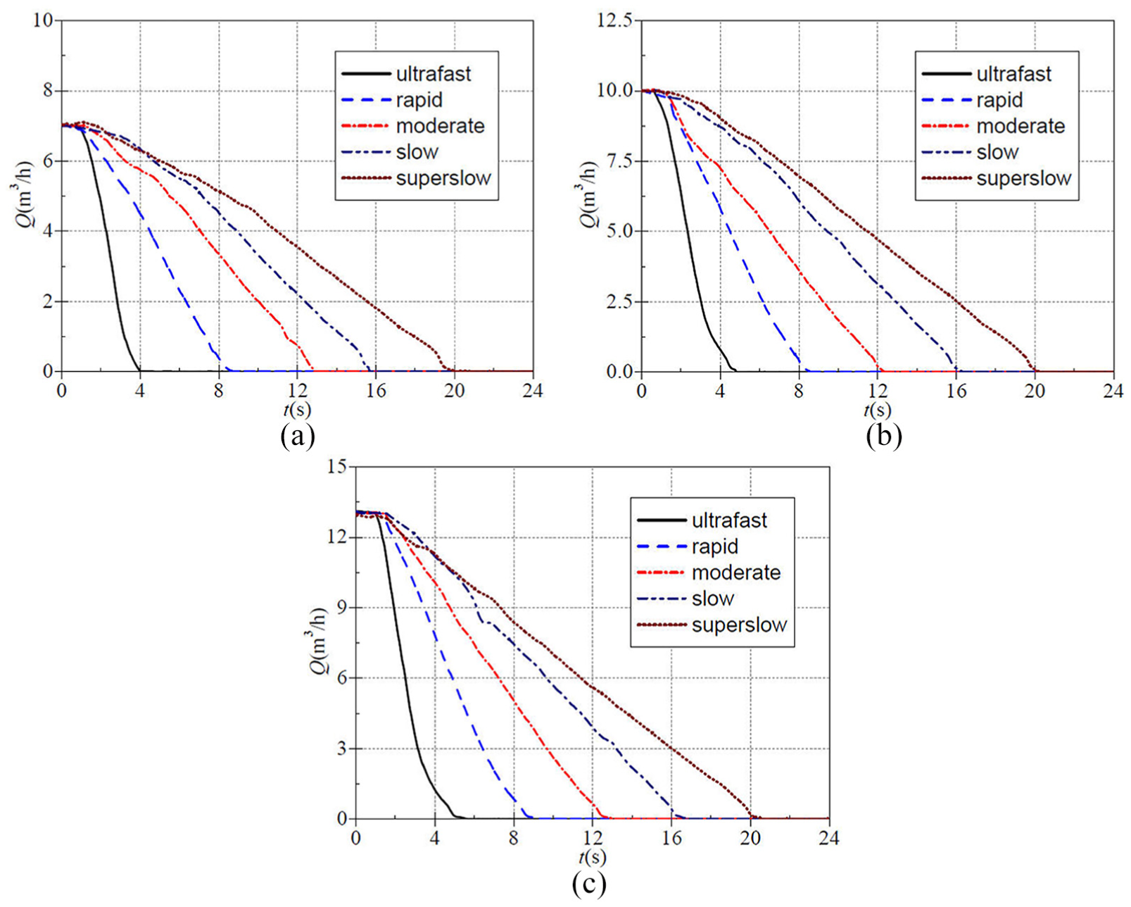
The time-history curves of the instantaneous heads measured during non-inertial stopping periods are shown in Figure 7. Although the static pressures at the pump inlet in Figure 5 vary considerably with time, the static pressures at the pump outlet in Figure 6 are much higher than those at the inlet; therefore, the static pressures at the outlet determine the magnitude of pump head essentially. Naturally, the static pressures at the outlet and the pump heads can share a similar profile in terms of time.

Figure 7.

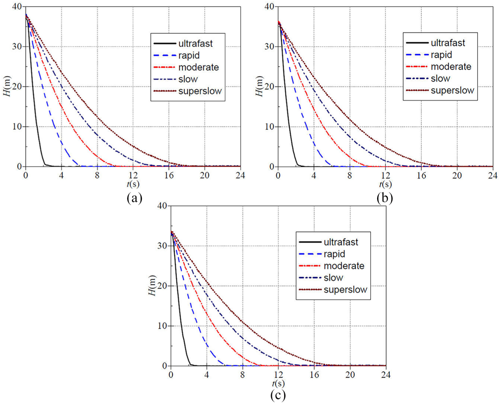
The instantaneous pump heads: (a) Q₀ = 7 m³/h, (b) Q₀ = 10 m³/h, and (c) Q₀ = 13 m³/h.

At the part-load, design, and over-load points, the average steady heads before stopping are 37.71, 35.98, and 33.13 m, respectively, showing a reducing tendency with increasing steady flow rate. Like the definition of λ_n and λ_Q, the head damping characteristic time (λ_H) is defined the ratio of the time (t_H) at 63.2% head drop to the time (T_H) at zero head.

At the part-load point of 7 m³/h, the ratios λ_H are 0.285, 0.378, 0.392, 0.380, and 0.390, respectively, at five non-inertial stoppings scenarios. At the design point of 10 m³/h, the ratios are 0.267, 0.342, 0.366, 0.361, and 0.381, and at the over-load point of 13m³/h, the ratios are 0.242, 0.329, 0.35, 0.357, and 0.380. Obviously, these ratios are decreased with increasing steady flow rate before stopping in every stopping scenario. This feature manifests that the pump head declines faster in the early and middle stage of non-inertial stoppings.

Shaft power

The recorded instantaneous shaft powers of the pump during non-inertial stopping periods are illustrated in Figure 8. The instantaneous rotational speed and shaft power were acquired through the torque detector; therefore, they are consistent in the time-history characteristics as shown in Figures 3 and 8.

Figure 8.

The instantaneous shaft powers: (a) Q₀ = 7 m³/h, (b) Q₀ = 10 m³/h, and (c) Q₀ = 13 m³/h.

At the part-load, design, and over-load points, the average steady shaft powers before stopping are 2.297, 2.302, and 2.310 kW, respectively, exhibiting a rising tendency with increasing steady flow rate before stopping.

Once more, the shaft power damping characteristic parameter (λ_P) is defined as the ratio of the shaft power damping characteristics time (t_P) to time (T_P) at zero shaft power. Since the rotational speed and the shaft power in experiments were synchronized, the ratios λ_n and λ_P are identical to each other in the same stopping scenario. Specially, in the ultrafast scenario of 1.0 s, λ_P is basically equal to 0.47. In the rapid stopping scenario of 3.0 s, λ_P is 0.60, but in the moderate, slow, and superslow stopping scenarios, λ_P is 0.62.

It turns out that no matter what the stopping scenario and the steady flow rate are, the three characteristic ratios are in an order such as λ_H < λ_P < λ_Q in terms of their values. This indicates that during non-inertial stopping periods, the head damping is the fastest, the shaft power damping is the moderate, and the flow rate damping is the slowest. The flow inertia of the liquid in the pipe system is responsible for this order.

Non-dimensional parameters

The non-dimensional flow rate, head, and shaft power are employed in order to better reveal the transient characteristics of the pump during non-inertial stopping periods. The non-dimensional parameters are defined as follows

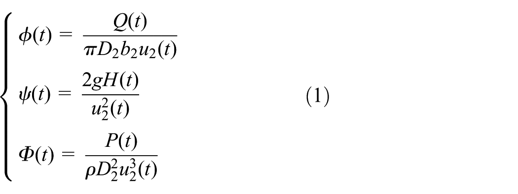
{\begin{matrix} ϕ (t) = \frac{Q (t)}{π D_{2} b_{2} u_{2} (t)} \\ ψ (t) = \frac{2 gH (t)}{u_{2}^{2} (t)} \\ Φ (t) = \frac{P (t)}{ρ D_{2}^{2} u_{2}^{3} (t)} \end{matrix}

(1)

where $u_{2} (t)$ is the instantaneous impeller speed at the impeller tip, $u_{2} (t) = π D_{2} n (t) / 60$ . Clearly, these non-dimensional parameters are independent of instantaneous rotational speed, and their time histories are demonstrated in Figures 9 –11, respectively.

Figure 9.

The instantaneous non-dimensional flow rates: (a) Q₀ = 7 m³/h, (b) Q₀ = 10 m³/h, and (c) Q₀ = 13 m³/h.

Figure 10.

The instantaneous non-dimensional pump heads: (a) Q₀ = 7 m³/h, (b) Q₀ = 10 m³/h, and (c) Q₀ = 13 m³/h.

Figure 11.

The instantaneous non-dimensional shaft powers: (a) Q₀ = 7 m³/h, (b) Q₀ = 10 m³/h, and (c) Q₀ = 13 m³/h.

Based on these figures, the non-dimensional flow rate, head, and shaft power curves have similar characteristics at any steady flow rate and in any non-inertial stopping scenario. At the beginning of non-inertial stopping, the three non-dimensional parameters are in the minimums, but they are not equal to zero value, and then almost keep constant with the increasing time. At the end of non-inertial stopping periods, the three parameters increase to the maximums rapidly. This variation characteristic during non-inertial stopping periods is significantly distinguished from that during inertial stopping periods shown by Tsukamoto et al.⁵ Meanwhile, this characteristic observed in the present testing is also found in the stopping period under frequency control by Wu et al.¹² In fact, the stopping under frequency control is non-inertial stopping. This fact establishes the advanced transient characteristic of the pump during non-inertial stopping periods but also manifests the remarked difference between inertial stopping and non-inertial stopping.

Discussions

The instantaneous head–flow rate curves are showed in Figure 12 for three steady flow rates. Meanwhile, the theoretical parabolic head–flow rate curves due to the affinity law for centrifugal pumps are also involved in the figure. In the present test schemes, the head and flow rate before a stopping are known. According to the affinity law of centrifugal pumps by Li and Zhang,¹⁹ the theoretical parabolic head–flow rate curves can be calculated using the following expression

H = H_{0} {(\frac{Q}{Q_{0}})}^{2}

(2)

where $Q_{0}$ and $H_{0}$ are the flow rate and pump head just before the stopping, Q is a measured flow rate during the stopping at a time moment, and H is the pump head calculated with a known Q.

Figure 12.

The instantaneous head–flow rate curves: (a) Q₀ = 7 m³/h, (b) Q₀ = 10 m³/h, and (c) Q₀ = 13 m³/h.

Initially, the experimental pump heads decrease rapidly. Subsequently, the pump heads begin to decrease slowly, and the curves approach to the theoretical parabolic profiles.

Note that the head–flow rate curve in the ultrafast stopping scenario of 1.0 s is obviously different from those of the other stopping scenarios. In other words, the curve is deviated most significantly from the theoretical curve. This implies that the affinity law for centrifugal pumps is no longer suitable to predict the transient performance in the ultrafast stopping scenario.

It is also found that four head–flow rate curves at the rapid, moderate, slow, and superslow stopping scenarios approach similar to the theoretical curve with increasing steady flow rate before stopping. Especially, the longer the stopping time, the more the head–flow rate curves close to the theoretical curve. This suggests that the affinity law can be used to estimate the transient performance of the pump in four scenarios, especially under the condition of large steady flow rate and in the superslow stopping scenario.

In this study, five linear rotational speed regulating patterns were prescribed, and the corresponding flow rate, head, static pressures, and shaft power responses were measured and illustrated in sections “Flow rate,”“Static pressure at inlet,”“Static pressure at inlet,”“Pump head,” and “Shaft power.” Since the shaft power is proportional to rotational speed, it shares the same time-history profiles with the prescribed speed patterns. The head and pump outlet static pressure responses are nearly the same and decrease with time. This agrees with the theoretical value in previous works.^13,20,21

For the inlet static pressure, there is a typical water hammer effect with over-shoot in its response curves. Specially, the shorter the stopping period, the larger the over-shoot.

The flow rate–time response curves are complicated in comparison with the others. Theoretically, its response to pump speed variations is decided by integrating the following energy equation with respect to time¹³

\frac{dq}{dT} + q^{2} - \frac{1}{{(β T + 1)}^{2}} = 0

(3)

where q is dimensionless flow rate, $q = Q / Q_{0}$ , T is the dimensionless time, $T = t / t_{1 / 2}$ , $β$ is the pumping system time constant ratio, $β = t_{1 / 2} / τ_{1 / 2}$ , $t_{1 / 2}$ is the time in which the system loop flow rate decreases to the half of its steady-state value, and $τ_{1 / 2}$ is the time in which the pump speed reduces to half of the steady-state value. Figure 13 demonstrates $q - T$ curves at various $β$ values in Gao et al.¹³ It is seen that the curves get steep with increasing $β$ value.

Figure 13.

$q - T$ curves at various $β$ values.

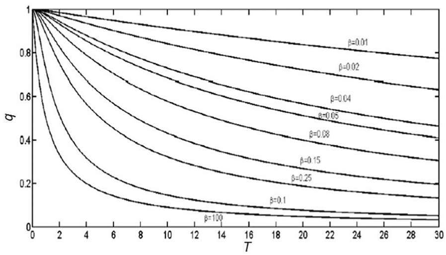
Based on Figures 3 and 4, the $β$ value gets large with shortening stopping time. For instance, at $Q_{0} = 10 m^{3} / h$ , β = 2.4 is in the superslow case, but β = 5.0 in the ultrafast case. It is considered that a gradually increasing $β$ in value results in a shaper flow rate curve when the stopping time becomes shorter and shorter.

Compared with the rotational speed time-history profiles, the flow rate response presents a delay or hysteretic phenomenon. This phenomenon may be caused from the slow response of the flow meter or the transient process itself. A confirmation study is needed. In the study, the instantaneous theoretical head and flow rate curves with stopping time will be calculated based on the measured rotational speed and the transient energy equation of the experimental rig. Then they will be compared with the measured instantaneous head–flow rate curves. Hence, the underlying mechanism of delay phenomenon in the flow rate will be identified.

Note that in this article, a pumping system without check valves was targeted. The underlying idea is regulating motor speed with a frequency converter to control pump stopping process to avoid pressure pulsation. Once the pump is fully stopped, the valves in the system will be closed. The results presented here are not applicable to the pumping system with check valves.

Conclusion

There is an obvious delay phenomenon in rotational speed decline at the end of non-inertial stopping when the stopping time is less than 3.0 s; and the shorter the stopping time, the more obvious the delay phenomenon. Meanwhile, it is also seen that there is an obvious delay phenomenon in the flow rate decline at the beginning of non-inertial stopping, but with increasing steady flow rate before stopping, the declines in both head and flow rate become faster.

The head damping is the fastest, the shaft power damping is the moderate, and the flow rate damping is the slowest. In the ultrafast stopping scenario, the static pressures at the inlet exhibit an oscillating pattern initially and then get flattened; further with the extension of the stopping time, this pattern disappears.

At the beginning of non-inertial stopping, the non-dimensional flow rate, head, and shaft power are in the minimums and then are almost keep constant with increasing time. At the end of the non-inertial stopping period, three non-dimensional parameters increase to the maximums rapidly.

The affinity law for centrifugal pumps is suitable to be used to predict the transient performance under the condition of large steady flow rate and in the superslow stopping scenario.

In the future works, the internal flow characteristics of pump during non-inertial stopping periods needs to be explored to reveal the underlying mechanism of time lag in head and flow rate.

Footnotes

Handling Editor: Jose Ramon Serrano

Declaration of conflicting interests

The author(s) declared no potential conflicts of interest with respect to the research, authorship, and/or publication of this article.

Funding

The author(s) disclosed receipt of the following financial support for the research, authorship, and/or publication of this article: The research was financially supported by the National Natural Science Foundation of China (grant nos: 51876103, 51536008) and the Zhejiang Provincial Natural Science Foundation of China (grant no.: LY18E090007).

ORCID iD

Yu-Liang Zhang

References

Weme

Schoot

Kruyt

et al . Prediction of the effect of impeller trimming on the hydraulic performance of low specific-speed centrifugal pumps. J Fluid Eng 2018; 140: 081202.

Zhu

et al . Experimental and numerical investigations of head-flow curve instability of a single-stage centrifugal pump with volute casing. Proc IMechE, Part A: J Power and Energy 2016; 230: 633–647.

Kim

Cho

Kim

et al . Design technique to improve the energy efficiency of a counter-rotating type pump-turbine. Renew Energy 2017; 101: 647–659.

Hao

Tan

Symmetrical and unsymmetrical tip clearances on cavitation performance and radial force of a mixed flow pump as turbine at pump mode. Renew Energy 2018; 127: 368–376.

Tsukamoto

Matsunaga

Yoneda

et al . Transient characteristics of a centrifugal pump during stopping period. J Fluid Eng 1986; 108: 392–399.

Lefebvre

Barker

WP.

Centrifugal pump performance during transient operation. J Fluid Eng 1995; 117: 123–128.

Thanapandi

Prasad

Centrifugal pump transient characteristics and analysis using the method of characteristics. Int J Mech Sci 1995; 37: 77–89.

Thanapandi

Prasad

A quasi-steady performance prediction model for dynamic characteristics of a volute pump. Proc IMechE, Part A: J Power and Energy 1994; 208: 47–58.

Tanaka

Tsukamoto

Transient behavior of a cavitation centrifugal pump at rapid change in operating conditions—part 2: transient phenomena at pump startup/shutdown. J Fluid Eng 1999; 121: 850–856.

10.

Rong

Tanaka

Ootsu

et al . Analysis of pump transient during starting/stopping periods by bond graph. JPN Society of Mechl Eng 1996; 62: 677–683.

11.

Liu

Wang

et al . Numerical simulation of the transient flow in a radial flow pump during stopping period. J Fluid Eng 2011; 133: 111101.

12.

Yang

et al . Transient characteristics of a closed-loop pipe system during pump stopping periods. J Press Vess Technol 2014; 136: 0211301.

13.

Gao

Zhao

et al . Transient flow analysis in reactor coolant pump systems during flow coastdown period. Nucl Eng Des 2011; 241: 509–514.

14.

Chen

et al . Analysis on transient performance of mixed flow pump during stopping period. Fluid Mach 2006; 34: 1–4.

15.

Wang

Yuan

Zhu

et al . Transient hydraulic characteristics study on nuclear reactor coolant pump during stopping period. Atomic Energy Sci Tech 2013; 47: 364–370.

16.

Zhang

Zhu

WG.

Experiments on transient performance of a low specific speed centrifugal pump with open impeller. Proc IMechE, Part A: J Power and Energy 2016; 230: 648–659.

17.

Zhang

Zhu

Sheng

et al . Experimental study on a prototype centrifugal pump with open impeller during stopping period. Int J Fluid Mech Research 2016; 43: 18–27.

18.

Zhang

Zhu

et al . Effects of viscosity on transient behavior of a low specific speed centrifugal pump in starting and stopping periods. Int J Fluid Mech Research 2018; 45: 1–20.

19.

Zhang

YL.

Centrifugal oil pump theory and application. Zhenjiang, China: Jiangsu University Press, 2016.

20.

Burgreen

Development of flow in a loop after pumping startup. Nucl Sce Eng 1960; 8: 277–278.

21.

Yokomura

Flow coastdown in centrifugal pump systems. Nucl Eng Des 1969; 10: 250–258.

Non-inertial stopping characteristics of a prototype pump

Abstract

Keywords

Introduction

Experimental pump, test rig, and method

Tested pump

Test rig

Experimental method and scheme

Results

Rotational speed

Flow rate

Static pressure at inlet

Static pressure at outlet

Pump head

Shaft power

Non-dimensional parameters

Discussions

Conclusion

Footnotes

Declaration of conflicting interests

Funding

ORCID iD

References