The study on tire tread depth measurement method based on machine vision

Abstract

The tire tread depth has strong influence on the braking performance of the vehicle and should be inspected periodically for driving safety. In order to determine the tire tread depth accurately and automatically, a tire tread depth measurement method based on machine vision was developed. During the measuring, a tire tread radial section image formed by a laser plane was captured when the tire rolls over the measuring device. Then, the image was calibrated to eliminate the lens distortion and processed to get the single-pixel center line. Consequently, the center line’s pixel coordinates were transformed to world coordinates with the calibration information of the laser plane, and a profile curve of the tire radial section was obtained. Then, the tread grooves on the profile curve were identified and their positions are determined by an algorithm developed in this research. Finally, the depth of each groove was calculated successively. An experiment was conducted on a prototype system based on the measurement method developed in this article. The experimental result indicates that the measurement method can identify the tire tread groove and determine its position and measure its depth. The depth absolute error is less than 0.2 mm, which can meet the demand of tire tread depth measurement.

Introduction

The role of the tire tread groove is to increase the friction between the tire tread and the road and to remove the water between the tire and the road to avoid slippage. For safety purpose, it is demanded that the vehicle’s tire tread depth could not be reduced below the limiting value. When the tread depth is below 1.6 mm, the tire should be replaced.

Traditionally, the tire tread depth is measured with a depth indicator when the vehicle is at rest. This kind of measurement is inefficient, human factor dependent, and inconvenient.^1,2 For the purpose of increasing the efficiency and reducing labor intensity, attempts have been made to facilitate the measurement of tire’s tread depth with image sensors.^3,4 Such devices consist of an array of laser light sources and multiple image sensors arranged in a line to acquire the tire’s profile. ³ Those systems reported do not involve automatic identification of the tire’s grooves. However, the identification of the grooves on the tire’s outer most surface is necessary for automatic measurement.

Huang et al. ⁵ developed a method for groove identification with a stereo vision system. The difference between the tire’s outer most surface and the bottom of the groove was identified by a Fuzzy C-means model. Thus, the grooves on the tire surface were identified. However, the tire’s tread depth error with the stereo vision system reached 1 mm in some cases. ⁵

Measuring technology based on structure light has been widely used for its stability and convenience.^6,7 The system on the tire’s tread depth measurement indicates that structure light measuring method can give satisfactory accuracy. ³ The realization of automatic identification of the grooves on a single tire section is necessary for the automatic measurement of the tire’s tread depth with machine vision and structure light.

In this article, a prototype tire tread depth measurement system is developed. Especially, a method for identifying the tire’s tread groove is introduced. When the tire rolls over the device, an image of the profile of the tire section formed by a laser plane intersection with the tire was captured. Then, the image is processed and calibrated to get the tire’s section profile curve. The grooves on the tire profile curve were identified, and the tire tread depth was measured. An experiment was conducted and the experimental results indicate that the measurement method can measure the tire tread depth automatically with acceptable accuracy.

Method for tire tread depth measuring with machine vision

Introduction of the measuring system

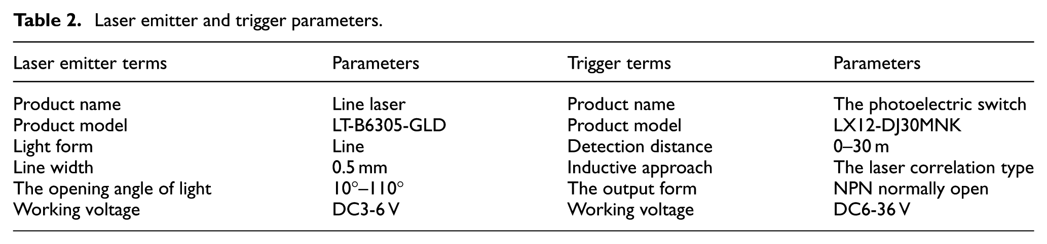
In the research, a prototype tire tread depth measuring system was designed as shown in Figure 1. The system consist of two cameras, two laser emitters, a reflecting mirror, a supporting plate, a trigger switch and the software based on LabVIEW. There are two windows on the supporting plate for the laser plane passing through and the reflecting mirror seeing the tire. Two cameras (the left camera and the right camera) are fixed under the supporting plate, and the camera’s principal axis is parallel to the ground and pointing to the mirror. The principal axis of the lens passes through the center of the mirror. The distance between the mirror center and the lens is 250 mm. With this distance, each camera has a view width of 250 mm with the selected focal length. Two cameras could cover a view width of 500 mm which is enough for the passenger car tire measurement. The parameters of the cameras are shown in Table 1. The mirror was placed for the cameras to see the image of the tire in the mirror. The angle between the mirror and the ground is 45°. The lasers adopted are line laser emitters, and the trigger adopted is a photoelectric switch. The parameters of the line laser emitter and those of the trigger are shown in Table 2. The main reason for the application of the line laser emitter is that the laser forms a laser plane and its projection is a line strip. The laser line width is 0.5 mm and the maximum opening angle of the laser emitter is 110°. Two line laser emitters can completely cover the tire tread surface, and two laser emitters were installed to form one laser plane. The laser plane is placed in front of the mirror, and the angle between the laser plane and the ground is 45°. The main reason that a photoelectric switch was applied is that the photoelectric switch’s trigger position on the supporting plate is a line. When the tire rolls over the supporting plate and passes by the photoelectric switch, the laser plane intersects with the tire tread and forms the tire radial section profile, and then, the cameras are triggered to capture the tire radial section profile image in the reflecting mirror.

Figure 1.

The schematic of the system.

Table 1.

Camera parameters.

Items	Left camera	Right camera
Sensor type	CCD	CCD
Sensor size	4.9 mm × 3.6 mm	4.9 mm × 3.6 mm
Resolution (H × V)	1294 pixels × 964 pixels	1294 pixels × 964 pixels
Pixel size (H × V)	3.75 µm × 3.75 µm	3.75 µm × 3.75 µm
Frame rate	30 fps	30 fps
Mono/color	Mono	Mono
Focal length	fx = 6.1 mm, fy = 6.1 mm	fx = 6.3 mm, fy = 6.2 mm
Optical center	u = 630.8 pixel, v = 491.4 pixel	u = 632.6 pixel, v = 452.1 pixel

CCD: charge-coupled device.

Table 2.

Laser emitter and trigger parameters.

Laser emitter terms	Parameters	Trigger terms	Parameters
Product name	Line laser	Product name	The photoelectric switch
Product model	LT-B6305-GLD	Product model	LX12-DJ30MNK
Light form	Line	Detection distance	0–30 m
Line width	0.5 mm	Inductive approach	The laser correlation type
The opening angle of light	10°–110°	The output form	NPN normally open
Working voltage	DC3-6 V	Working voltage	DC6-36 V

The tire radial section profile records the tire tread depth and groove numbers. If the laser plane passes through the center of the tire rotation axis, the depth of the groove on the tire radial section profile equals to the real tire tread depth, otherwise the measured depth of the grooves on the image is bigger than the real tire tread depth. The difference between them increases with increasing distance between the laser plane and the tire axis. When the position of the trigger switch on the supporting plate is fixed, the distance from the laser plane to the tire axis varies with changing tire diameter. In this article, a model which can get the real depth from the measured depth for different tire diameters is built. The model is the basis for the measuring method in this research.

The laser plane intersects with the tire tread and gets the tire radial section profile. When the tire rolls over the supporting plate and passes the photoelectric switch, the camera is triggered, and the tire radial section profile image was obtained. The tire radial section profile records the tire tread depth and groove numbers. If the laser plane passes through the center of the tire rotation axis, the depth of the groove on the tire radial section profile equals to the real tire tread depth, otherwise the measured depth of the grooves on the image is not equal to the real tire tread depth. The difference between them is determined by the relative position between the tire and the laser plane. Determining the relative position between the laser plane and the tire is the foundation of tire tread depth measurement.

Mathematical model of the measuring system and analysis

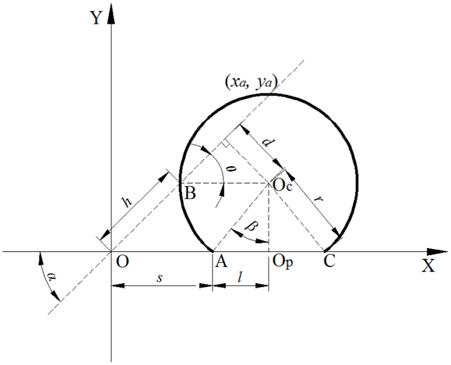
With standard tire pressure, there is a slight variation in the dimension of the tire tread in the tire radial direction except for the ground contact area. The laser plane projects on the tire surface which is far from the contact area. So, the tire tread can be simplified to a cylindrical surface. Projecting the laser plane and the tire tread along the tire axis direction, the diagrammatic sketch of the measuring system is obtained and shown in Figure 2. The beam OB is the projection of the laser plane. The arc ABC is the projection of the tire tread. Line segment AC is the projection of the tire contacting with the ground. Line AC is the projection of the ground. O_c is the projection of the tire rotation axis. Take O as the origin and establish the coordinate system shown in Figure 2. The angle between OB and OA is α. The angle between OB and BO_c is θ. The length of OA is s, the length of AO_p is l, the distance between O_c and OB is d, and the length of OB is h.

Figure 2.

The schematic of the test.

In the coordinates established, the coordinates of O_c are

$$x_{O_c}=s+l$$

(1)

$$y_{{\mathrm{O}}_{\mathrm{c}}}=\sqrt{r^2-l^2}$$

(2)

The equation of arc ABC can be given by

$${(y-\sqrt{r^2-l^2})}^2+(x-s-l{)}^2=r^2(y>0)$$

(3)

The equation of beam OB is

$$y=x·\tan \alpha$$

(4)

The intersection of beam OB and arc ABC is B. And the coordinates of B meet

$${(x_B·\tan \alpha -\sqrt{r^2-l^2})}^2+{[x_B-(s+l)]}^2=r^2$$

(5)

From expression (5), the relationship between tire radius r and the coordinate x_B satisfies

$$\sqrt{r^2-l^2}=\frac{x_B^2·{\left(\tan \alpha \right)}^2-l^2+x_B^2-2(s+l)·x_B+{(s+l)}^2}{2·\tan \alpha ·x_B}$$

(6)

From equation (4), the relationship between coordinate x_B of point B and h could be deduced

$$x_B=h·\cos \alpha$$

(7)

Plugging expression (7) into expression (6), an expression of radius r, measured distance h, and the contact length l satisfies

$$r^2={\left[\frac{h^2-l^2-2(s+l)·(h·\cos \alpha )+{(s+l)}^2}{2·h·\left(\sin \alpha \right)}\right]}^2+l^2$$

(8)

The angle between OB and BO_c is

$$\theta =a\sin \left(\frac{\tan \left(\alpha \right)(s+1)-\sqrt{r^2-1^2}}{\sqrt{1+{\tan }^2\left(\alpha \right)}}\right)$$

(9)

θ is a function of s, l, h, and α

$$\theta =a\sin \left(\frac{\tan \left(\alpha \right)(s+l)-\left[\frac{h^2-l^2-2(s+l)·(h·\cos \alpha )+{(s+l)}^2}{2·h·\left(\sin \alpha \right)}\right]}{\sqrt{1+{\tan }^2\left(\alpha \right)}}\right)$$

(10)

The measured tread groove depth on the image and the real tire tread depth satisfy

$$\mathrm{\Delta }{H}_R=\mathrm{\Delta }{H}_M·\cos \theta$$

(11)

For a specific tire with standard tire pressure, the angle β is affected by the load on the tire. Angle β is bigger when the load is heavier. During the measurement, the vehicle is demanded to bear specific load and the angle β is nearly constant. Then, l is nearly a constant for a specific vehicle. When l is constant, the relationship between radius r, the spacing s, and the measured distance h is shown in Figure 3. With the same distance s, the measured distance h decreases with the increase in the radius r. There is an one-to-one correspondence between the measured distance h and the radius when s is a constant. With the same radius r, the measured distance increases with the increase in distance s. The difference Δh between the measured distances h of the 0.2 m radius tire and that of the 0.45 m tire increases with the increase in the spacing s. The numerical calculation of the model indicates that when the distance s is 0.25 m, the measured distance difference Δh is about 0.1 m. The laser strip between this distance difference Δh can be reflected completely in the mirror window. The laser strip image of the tires whose radius is in the range from 0.2 to 0.45 m could be captured. A narrow sensing area can be used to save the pixel resources of the camera with acceptable measuring accuracy.

Figure 3.

S-R-h relationship.

Figure 4 presents the relationship between angle θ, the distance s, and the radius r. In the radius range considered, when distance s is a constant, the angle θ decreases with increasing radius near linearly. When the radius r is constant, the angle θ increases with increasing s. When s = 0.25 m, the angle θ changes from about 6° to about −5° with increase in the radius r from 0.2 to 0.45 m.

Figure 4.

S-R-A relationship.

Figure 5 shows the relationship between the tire radius r, the distance l, and measured distance h when s is constant. With the same h, the corresponding radius r increases with the nearly linear increasing distance l. When l is constant, the radius r increases with increasing measured distance h. At the maximum tire radius 0.45 m, the measured distance h is about 0.1 m. When l has a change of 0.02 m, it implies about 0.05 m change in radius r. From Figure 4, it can be found that when there is a difference in radius below 0.05 m, the difference in angle is less than 4°. The difference in angle of 4° can cause an error of 0.039 mm when the tire tread depth is 16 mm. When the range of distance l is limited to 0.02 m, the effect of l change on the depth can be neglected.

Figure 5.

H-L-R relationship.

Figure 6 shows that the angle θ changes with the distance l when s is constant and h is a variable parameter. When h equals 0.1, the ratio of angle θ and distance l is maximum. When l has a change of 0.02 m, there is a change in the angle of less than 4°. The analyses of Figures 4 and 5 are confirmed.

Figure 6.

H-L-A relationship.

In summary, the angle between the laser plane and the tire radius can be determined by measuring h and l. When the changing range of θ caused by the change in l is less than 4°, the change in l caused by the depth error is smaller than the system’s resolution. In some cases, l can be taken as constant with acceptable error. The changing range of l studied can cover the change in the real contact distance of the corresponding tires caused by the tire pressure deviating from standard value. It indicates that the measuring method presented here can get acceptable accuracy even l has a small change due to the tire pressure deviation.

The tire profile laser strip image processing

The purpose of image processing here is to get the laser strip center line presented in world coordinates from the captured tire radial section profile image. The work flow of image processing is shown in Figure 7.

Figure 7.

The work flow of image processing.

When the tire reached the trigger switch, the left and the right cameras are triggered to capture the image simultaneously. The cameras are controlled with a program based on LabVIEW vision module. Each camera captures a part of the tire surface as shown in Figure 8. Two images cover the whole width of the tire surface. The white strip in each image is part of the tire section profile formed by the laser projection.

Figure 8.

The photograph from the (a) left camera and (b) right camera.

Before measuring, the position of the laser plane relative to the cameras is determined according to previous studies.^8,9 The laser plane is treated as a planer pattern. Its position relative to the camera is described by a rotation matrix and a translation vector (the extrinsic parameters). ¹⁰

With the intrinsic parameters of the camera, the images are calibrated to remove lens distortion. ¹⁰ Then, the images are filtered to eliminate noise with a Gaussian filter whose window size is 16 × 16. ¹¹ Consequently, the images are segmented by illumination to extract the laser strip in the image. The extracted laser strips from the two cameras are shown in Figure 9.

Figure 9.

The segmented image from the (a) left camera and (b) right camera.

In Figure 9, the pixel value is set to zero except for the pixels in the laser strip. The tire and the surrounding images are removed and only the laser strip is left on the image. ¹² The shape of the laser strip on the image is relatively simple and the center line of single pixel (Figure 10) was obtained by grayscale barycenter method. ¹³

Figure 10.

The center line of the strip in the image from the (a) left camera and (b) right camera.

The center line’s world coordinates (Figure 11) are obtained by transforming the center line’s pixel coordinates to world coordinates with the extrinsic parameters of the laser plane in the software developed based on LabVIEW.^9,10,14 The center line from the left camera gives a complete view of the tire’s left shoulder as shown in Figure 11(a). The center line from the right camera gives a view that includes the complete right shoulder of the tire as shown in Figure 11(b). The right side of the center line from the left camera is overlapped with the left side of the center line from the right camera. So, the center line from the two cameras together gives a complete view of the tire’s section profile.

Figure 11.

The curve of the (a) left camera image and (b) right camera image.

The laser strip center line in world coordinates represents the tire radial section profile. The origin of the world coordinates system is determined by the origin of the laser plane which is designated during laser plane position determination. The shape of the center line and the relative position of two points on the center line do not change with the change in the origin. The tread position and depth on the center line in world coordinates is one-to-one correspondent to the real tread groove position and depth on the tire. The tire tread depth can be measured on the center line of world coordinates.

Tire tread identification and depth measurement

The identification of the tire tread groove on the laser strip center line of the world coordinates system is the key of automatic measuring. The tread groove identification includes determining the tread groove characteristics and determining the grooves’ locations and numbers. After tread identification, the measurement of each tread groove’s depth is done successively.

The tread groove characteristic determination

Combine the center line coordinates array from two cameras together. The whole laser strip center line of world coordinates array was obtained. Because the laser strip brightness is uneven, the x coordinates of the center line is not equally distributed. For the convenience of data processing, the combined center line coordinates array was interpolated to get a new array whose x coordinates were equally distributed. The tire radial section profile curve in the new coordinates was shown in Figure 12. The abscissa spacing is taken as 0.5 mm, which could present the shape of the tire radial section profile without unacceptable detail loss.

Figure 12.

The interpolation curve.

It can be found in Figure 12 that the tire tread groove was characterized as concave on the tire radial section profile curve. For the reason that there exists test error and there are smaller scale grooves on the tire tread surface, there are some smaller concaves on the tire radial section profile curve except for the concave from the tire tread groove. It is necessary that the algorithm can distinguish the concave from the tire tread groove and the concave from other sources during the tire tread groove identification.

The smaller concave can be removed from the profile curve by applying the Gaussian filters on the curve. When the scale σ of the Gaussian function is applied, the concave of the corresponding scale on the profile curve can be strengthened. One task of the tread groove identification is to select proper scale Gaussian functions. The discrete Gaussian function of scale σ_k can be expressed as

$$g_{\mathrm{ki}}=\frac{1}{{\sigma }_k\sqrt{2\pi }}{e}^{(-\frac{{x_i}^2}{2{{\sigma }_k}^2})}$$

(12)

The convolution of the discrete Gaussian function and the tire radial section profile curve is

$$Y=y_i*g_{\mathrm{ki}}$$

(13)

Figure 13 shows the results of the convolution of the profile curve of tire 175/70r14 and the discrete Gaussian function of scales σ_k = 1, 3, 5, 7, 9, 11, and 13; the domain of the discrete Gaussian function is x_i ∈ (−3σ_k, 3σ_k) and Δx_i = 0.5. It can be found that there is still some obvious convex except for that from the tire tread groove when scale σ_k < 5. When the scale σ_k > 11, the convex from the tire tread groove was smoothed away.

Figure 13.

The filtered curve.

The local maximum extreme points on the filtered curve by Gaussian function of scales σ = 3, 9, and 13 are shown in Figure 14. When σ equals 3 or 13, there is no one-to-one correspondence between the local maximum extreme points and the tread concave. When σ = 9, the maximum extreme points and the tread concaves are one-to-one correspondent by taking the maximum extreme point at the left side of the groove. The calculation results showed that when σ belongs to 5–11 range, there is one maximum extreme point on each side of a tread groove, and the one-to-one correspondence between the maximum extreme points and the concave can be established by taking the maximum extreme point at one side of the groove.

Figure 14.

The extreme value point distribution of σ.

For the 235/50R18 tire, it has three circumferential grooves, and the radial section profile curve is shown in Figure 15. The convolution of the 235/50R18 radial section profile curve and the discrete Gaussian function of scale σ_k = 1, 3, 5, 7, 9, 11, and 13 are shown in Figure 16. When σ = 3, the convolution curve is smooth enough to eliminate the small concave from the test error or the smaller grooves. When σ > 5, some concave from the tire tread groove has been smoothed away. The local maximum extreme points on the filtered curve by Gaussian function whose scale σ = 1, 3, 5, 7, and 11 are shown in Figure 17. When σ > 5, there is no one-to-one correspondence between the local maximum extreme points and the radial section profile curve concave.

Figure 15.

The interpolation curve.

Figure 16.

The filtered curve.

Figure 17.

The curve and the convolutions with different σ: (a) σ = 1, (b) σ = 3, (c) σ = 5, (d) σ = 7, and (e) σ = 11.

For the other ordinary tires, the testing indicates that when σ = 5, the one-to-one correspondence between the tread concave and the local maximum extreme points can be established. The tire tread groove can be identified with the discrete Gaussian function whose scale is 5. When the tread groove is identified, the location of the tread groove and the number of the tread groove are clarified.

The measure of the tread depth

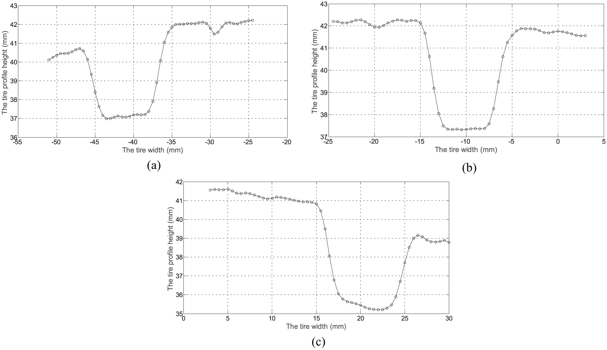
After the clarification of the tread groove location and number, the depth of each tread groove can be measured successively. Between two local maximum extreme points on the convolution curve, there is a tread groove. Each tire tread groove curve extracted from the tire profile curve from 175/70r14 tire and 235/50R18 tire is shown in Figures 18 and Figure 19, respectively. The measured depth of each tire tread groove is the maximum of the distances from the bottom of the concave to the line ending on each side of the concave. The depth is calculated by the following steps:

1. Select the curve for one tread groove. Find the point with minimum y value and record its coordinates (x_B, y_B); for convenience, give the point a name: B.

2. On each side of B, find points with maximum y value and recorded as L and R and record their coordinates (x_L, y_L) and (x_R, y_R).

3. Test whether all the points on the curve are under LR. If so, proceed to next step; if not, take the highest point as new L or R points.

4. Calculate the distance from B to line LR. Then, the location and depth of the tread groove are obtained.

5. Repeat steps (1)–(4) until all the tire tread groove depths are calculated.

Figure 18.

Single-groove curve of 175/70R14 tire: (a) the first groove from the left, (b) the second groove from the left, (c) the third from the left, and (d) the fourth groove from the left.

Figure 19.

Single-groove curve of 235/50R18 tire: (a) the first groove from the left, (b) the second groove from the left, and (c) the third groove from the left.

There is a difference between the measured depth and the real depth when the laser plane does not pass through the tire’s axis as mentioned in section “Mathematical model of the measuring system and analysis.” The real depth can be obtained with the measured depth by following steps: (1) calculate l with the measured h and the known r by expression (8); (2) calculate the angle θ by expression (9) or (10); and (3) calculate the real depth with the measured depth by expression (11). The abovementioned steps are implemented in a LabVIEW program developed in this research.

Experimental results

To verify the measurement method, experiments were conducted on two tires. A LabVIEW program based on its vision module is developed in this research. The algorithms developed are implemented in the software. When the tire rolls over the supporting plate, the tire groove’s number and position are found, and the depth is calculated by the LabVIEW program. The experimental results found that the system can capture the tire tread section laser strip profile, and the algorithm can identify the tread groove and measure its depth. The picture of the depth gauge is shown in Figure 20, and the measurement method using the depth gauge is shown in Figure 21. The precision of the tire using depth gauge is 0.01 mm, and it can satisfy the measurement accuracy. The measurement method based on the machine vision is shown in Figure 22, and the measuring interface based on the machine vision is shown in Figure 23. The measurement results from the machine vision and the results from the depth gauge are shown in Table 3. The measured results of the depth gauge are the average value of the three times of measurements. The experimental results indicated that the measurement system could identify the tread groove and measure its depth automatically. The maximum percentage error is 2.47% and the minimum percentage error is 0.41%. All the errors are less than 0.2 mm, and the test could meet the demand of tire tread depth measurement.

Figure 20.

The depth gauge.

Figure 21.

The measurement method using the depth gauge.

Figure 22.

The measurement method based on the machine vision.

Figure 23.

The measuring interface based on the machine vision.

Table 3.

The comparison of results from the machine vision and the depth gauge.

175/70R14					235/50R18
Items	Machine vision	Depth gauge	Percentage error	Absolute error	Machine vision	Depth gauge	Percentage error	Absolute error
The number of tread	4	4			3	3
The first tire groove depth from the left	4.75 mm	4.80 mm	1.04%	0.05 mm	4.74 mm	4.7 mm	0.85%	0.04 mm
The second tire groove depth from the left	5.33 mm	5.41 mm	1.48%	0.08 mm	4.71 mm	4.68 mm	0.64%	0.03 mm
The third tire tread depth from the left	5.53 mm	5.48 mm	0.91%	0.05 mm	4.56 mm	4.45 mm	2.47%	0.11 mm
The fourth tire groove depth from the left	4.80 mm	4.82 mm	0.41%	0.02 mm

Conclusion

A new tire tread depth measurement method based on machine vision is presented in this article. Based on the mathematical model and the identification algorithms developed, the measuring processing consists of image capturing and processing and the identification and the depth calculation of the grooves. The experiment indicates that tire tread groove can be identified and the depth can be measured. The details are as follows.

1. The measurement system developed can capture the rolling tire’s radial section profile image. The image processing and calibration can obtain the tire’s section profile curve.

2. The tire tread groove identification method and the depth measurement algorithm can identify the tread groove and measure its depth. The algorithms can be implemented in a program developed based on LabVIEW vision module.

3. Experiment was conducted on a prototype system. The experiment indicates that the tire tread groove was identified and the depth was measured automatically. The absolute error is less than 0.2 mm. The system can meet the demand of tire tread depth measurement.