Experimental study and numerical simulation of propagation and coalescence processes of pre-existing flaws in a transparent rock-like material

Abstract

Flaws in the rock play an important role in the failure of rock engineering. In this article, some rock-like specimens prepared by transparent resin material were used to investigate the propagation and coalescence processes of pre-existing closed three-dimensional flaws, and a series of uniaxial compressive tests were carried out to study the effects of flaw dip, flaw area, flaw friction coefficient, and composite flaw spacing on mechanical properties and flaw propagation and coalescence processes. Based on the particle flow method, the experimental results were verified by numerical simulation. The results show that there is a good agreement on flaw propagation rule revealed by the experiments and numerical simulations. In the case of the specimens with single-flaw, with the increase of the inclination angle, the peak stress of the specimen first decreases and then increases, when the inclination angle is 45°, the peak stress is the smallest. Meanwhile, the peak stress decreases with the increase of flaw area but increases with the increase of flaw friction coefficient. The spacing of the composite flaw has a significant influence on the strength, and the impact on the elastic modulus is not obvious. The results can provide a reference for the mechanism of flaw propagation and coalescence.

Introduction

Rocks in nature have undergone long-term geological processes, usually containing micro-scale features such as different scales and randomly distributed fractures, which have a very important influence on the strength and stability of rock mass. The failure of large rock mass construction has a very close relationship with propagation and coalescence processes of its internal flaws.

At present, many methods have been adopted by scholars to study the propagation and coalescence of internal flaws in rock mass, mainly including experimental tests and numerical simulations. For instance, Bobet and Einstein ¹ used gypsum specimens to simulate rock under uniaxial and biaxial compression; according to the different shapes and sizes of pre-existing flaws, they proposed three failure patterns including the combination of wing flaw and secondary flaw. Wong and Chau ² also categorized the flaw coalescence patterns in nine cases from the results of a series of uniaxial compression test. Sagong and Bobet ³ made 3 and 16 flaws in gypsum specimens and carried out uniaxial compression tests to observe the coalescence patterns in double-flawed specimens to be extrapolated to multiple flawed specimens. Lee and Jeon ⁴ used three different types of specimens containing single- and double-flaws to study the failure pattern under uniaxial compression. Manouchehrian and Marji ⁵ studied the flaw propagation and failure process under the biaxial compression in the rock-like materials. The results show that the direction of the secondary flaw is related to the material type and the restraint stress. In addition to the experimental work, the computed tomography (CT) scanning test was used to study the effect of pre-existing flaws number and dip on the strength and failure patterns under uniaxial compression and three-dimensional (3D) single-flaw propagation mechanism by Tian and Han ⁶ and Ge et al. ⁷

Many numerical methods have also been developed to simulate flaw initiation and propagation. These numerical methods include the finite element method (FEM), general particle dynamics (GPD), and discrete element method (DEM). ⁸ Areias and Belytschko ⁹ used the extended FEM to analyze the 3D flaw initiation and propagation. Based on the FEM, the simulation of rock internal flaw growth was carried out by Prabel et al.; ¹⁰ compared with the test results, the numerical simulation results are in good agreement with the test results. Fu and colleagues^11,12 established a kind of elastic-brittle constitutive model with FLAC3D ¹³ while tests with resin material and numerical simulations were carried out. In addition, a new meshless algorithm was used to conduct a numerical simulation study of rock-like materials by Zhou et al., ¹⁴ Bi et al., ¹⁵ and Wang et al. ¹⁶ The numerical results are in good agreement with the experimental results. As for DEM, the bonded particle model (BPM) was used to simulate rock material and flaw propagation by Potyondy and Cundall, ¹⁷ Potyondy, ¹⁸ and Cho et al.; ¹⁹ the experimental results were in good agreement with the numerical simulation results. The parallel bond model was used to simulate the pre-existing closed 3D flaws under uniaxial compression by Zhang and Wong^20,21 and Lisjak and Grasselli. ²² The results show that the inclination angle, length and rock bridge angle play an important role in different failure modes.

In this study, the transparent resin material was used to prepare rock-like specimens, and a series of uniaxial compression tests were carried out to study the effects of flaw dip, flaw area, flaw friction coefficient, and composite flaw spacing on the mechanical properties of the rock-like samples and flaw propagation. Based on numerical simulation by the particle flow code in two dimensions, the mechanism of initiation and propagation of flaws in the rock-like sample was revealed from the mesoscopic perspective.

Experimental tests of transparent rock-like material with pre-existing flaws

Preparation of transparent rock-like specimens

In nature, rock mass is non-transparent material, and it is difficult to observe the propagation of its internal flaws under normal circumstances. Hence, in this work, a new transparent brittle resin material and additives were used to prepare transparent rock-like specimens in order to clearly observe the propagation process of flaws. Considering the advantages of quick solidification, smooth surface, low shrinkage, and so on, an unsaturated polyester resin was employed. Meanwhile, the ratio of additives was constantly adjusted during the specimen preparation process to make the mechanical properties of rock-like specimens close to the actual rock. At room temperature, the tension–compression ratio of the prepared specimen can be 1/5, even reach 1/7 at −50°C. Because of the significant brittle characteristics, the process of rock failure can be shown more reasonable.

Figure 1 shows the preparation process of a rock-like specimens, including the following steps:

1. According to the ratio proportion, a certain amount of liquid resin, curing agent, and other additives were poured together into the beaker, stirring slowly for 5 min to prevent the impact of the bubble on test results.

2. The prepared resin liquid was poured into the mold, which was a cuboid with pre-existing flaws hanging in it. The liquid was poured down along the mold wall slowly to ensure that no bubbles generated. Then the mold was placed horizontally for over 24 h at room temperature.

3. Because of the unsaturated resin from the liquid into solid, the volume will decrease, causing the specimen surface to sag. The surface of the sample was polished to make the sample to be a cuboid.

4. After polishing, the specimens were placed in the oven for five times. It takes about 30 min to make it fully solidified during each baking. After baking, the specimens were moved for storage at low temperature to ensure its brittleness.

Figure 1.

A kind of new unsaturated resin material: (a) pre-flawed rock with a certain inclination angle, (b) rock with a horizontal flaw, (c) rock with two flaws after uniaxial compression, and (d) the configuration material of a transparent rock.

According to the uniaxial compression tests result of the intact rock-like specimen, the density of the specimen is 1910 kg/m³, Young’s modulus is 6.3 GPa, the uniaxial compressive peak stress is 98.7 MPa (as shown in Figure 2), and the tensile strength measured by Brazilian split test is 17.9 MPa. A mica sheet of 0.1 mm thickness was used to simulate an oval pre-existing flaw in the specimen, and the pre-existing flaws were fixed in the mold with a certain inclination angle.

Figure 2.

Stress–strain curve of intact rock-like specimen under uniaxial compression tests.

Uniaxial compression tests of single-flaw specimens

In order to study the effects of flaw dip, flaw area, and flaw friction coefficient on the mechanical properties and failure patterns of single-flaw specimens, several different specimens were prepared, and a series of uniaxial compression tests were carried out to investigate the evolution process of flaws and failure patterns of fractured rock.

The analysis of failure process of single-flaw specimen

During the uniaxial compression tests, the failure process was recorded by a Sony NEX-VG900 camera. Taking the single-flaw specimen with 60° inclination angle as an example, the failure process under uniaxial compression was analyzed as follows. Figure 3 shows the failure process of the specimen under uniaxial compression. It can be seen from Figure 3 that the flaw initiation stress of the specimen is between 45% and 55% of the peak stress, and some secondary flaws start to appear at the edge of long axis of the elliptical flaw, and then flaws rapidly expand into petal-like flaws as the loading continues. The petal-like flaws cease to grow along the length direction of the flaw at a certain moment when the petal-like flaws fully develop, and the flaws are gradually wrapped around the flaw. Then, the stress is released at the weak parts around the flaw until the stress reaches about 80% of the peak stress. At this point, petal-like flaws develop into wing flaws. The wing flaws grow gradually along the length direction and turn toward the loading direction, but the growth rate is extremely slow. When the load reaches about 90% of the peak stress, the second sudden expansion of wing flaws appears along its length direction, and the length of the expansion is longer than that of the first expansion. The final growth length of wing flaws is about two to three times short axis of flaw. As the load continues to increase, the intact area begins to produce micro-flaws and these flaws coalesce until destruction. The final failure of the specimen is mainly caused by the expansion of the wing flaws, and the failure pattern is the tension and splitting destruction.

Figure 3.

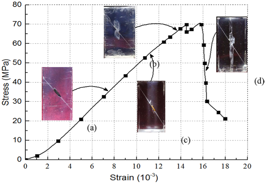
Stress–strain curve of specimen with 60° dip flaw: (a) the beginning of the flaw initiation, (b) the petal flaws, (c) the wing flaws, and (d) tension splitting destruction of the wing flaws.

The effect of flaw dip on the mechanical properties of specimens

As shown in Figure 4(a), the stress–strain curves of the specimens with single-flaw of different inclination angles, 15°, 30°, 45°, 60°, and 75°, were obtained by uniaxial compression tests, respectively. From Figure 4(b), it can be found that the peak stress and the flaw initiation stress decrease first and then increase with the increase of the inclination angle. When inclination angle is 45°, the peak stress and the flaw initiation stress both reach their minimum values. Moreover, changes in the amplitude of the peak stress and the flaw initiation stress are different, and the variation of the flaw initiation stress is relatively small compared with the peak stress.

Figure 4.

Mechanical properties of uniaxial compression with different inclination angles: (a) the stress–strain curve of the specimen with different flaws and (b) the peak stress and the initiation stress.

The effect of flaw area on the mechanical properties of specimens

The effect of different flaw areas on the propagation and coalescence processes was studied by uniaxial compression tests. Taking the specimen with 45° inclination angles as an example here, the specimens were divided into seven groups according to the different area of flaws, and the flaw areas are 0 (intact specimen), 131.1, 201.1, 314.3, 452.4, 615.8, and 804.2 mm². The stress–strain curves of the specimens are shown in Figure 5(a).

Figure 5.

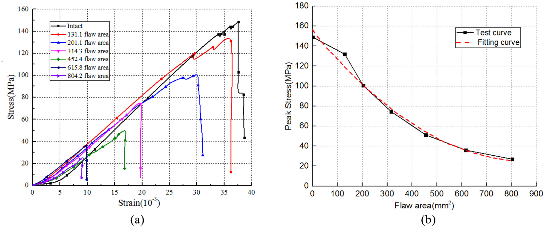
Mechanical properties of uniaxial compression with different flaw areas: (a) the stress–strain curve of the specimen and (b) the peak stress of the specimen with different flaw areas.

According to the correspondence between pre-existing flaw area and peak stress, the variation rule of flaw area and peak stress is summarized in Figure 5(b). It can be seen from Figure 5(b) that the change trend of peak stress is very rapid with flaw area from 0 to 200 mm², while the flaw area is 800 mm², the change trend of peak stress is quite gentle. It shows that with the increase in the flaw area, the peak stress gradually decreases, and the change trend slows down, indicating that the strength of the specimen decreases.

The relationship between the peak stress and the flaw area of the specimen is roughly represented by a quadratic function, whose expression is as follows

$$\sigma =b+a_{1}s+a_2{s}^2$$

(1)

where $\sigma$ is the peak stress, $s$ is the flaw area, b = 154.87 MPa, a₁ = −0.3 MPa/mm², and a₂ = 1.74 MPa/mm⁴.

The effect of coefficient of friction on the mechanical properties of specimens

Rock flaws in nature are often filled with impurities. The different impurities in flaws and the different material properties of the rock itself lead to differences in the friction coefficient of flaws. The copper slice, mica slice, and plastic slice (polyethylene) were used as flaws, and the different friction coefficient of flaws were characterized by the friction coefficient of three materials. The friction coefficients of the materials are shown in Table 1. The stress–strain curves of the specimens are shown in Figure 6(a), and the relationship between the friction coefficient and the peak stress is shown in Figure 6(b).

Table 1.

Different contact surface friction factor.

Contact surface type	Copper–resin	Mica–resin	Polyethylene–resin
Friction factor	0.21	0.18	0.12

Figure 6.

Mechanical properties of friction coefficients for different contact surface: (a) the stress–strain curve under different friction coefficients and (b) the peak stress of different friction coefficients.

It can be seen from Figure 6(a) that the peak stress increases with the increase in the friction coefficient of the specimen, which indicates that with the increase of the friction coefficient, the strength of the specimen increases and the stability is also improved, the relationship between the peak stress and the friction coefficient of the flaw surface is basically linear, as shown in equation (2)

$$\sigma =b+\mathrm{af}$$

(2)

where $\sigma$ is the peak stress and $f$ is the friction coefficient. The values of $a$ and $b$ were derived by linear fitting as follows: a = 273.71 MPa, b = 26.49 MPa.

Uniaxial compression tests of double-flaw specimens

For the double-flaw specimens, the influence of the flaw spacing on the mechanical properties was considered. The specimens were divided into four groups according to the different flaw spacings, and the flaw spacings are 10, 20, 30, and 40 mm, respectively. The directions of the two flaws are parallel to each other, and the connecting line between the lowest point of the upper flaw and the highest point of the lower flaw is perpendicular to the flaws, and the center of the connecting line is the center of the specimen. The single factor analysis method was used to make sure that the shape, size, and inclination angle of the flaw in the specimen remained unchanged, and in this case, the inclination angle was set to 60°. It can be seen from Figure 7 that the peak stress of the specimen decreases gradually as the flaw spacing increases. The peak stress of specimens with flaw spacing of 10, 20, 30, and 40 mm are 61.15, 58.39, 56.47, and 53.53 MPa, respectively, decrease by 34.79%, 37.74%, 39.78%, and 42.91%, respectively, compared with 93.78 MPa of intact specimen. The flaw spacing has a significant effect on the compressive strength of the specimen. It can be seen from Table 2 that the amplitudes of elastic modulus and the flaw initiation stress of the specimen are small, and the variation law is not obvious. It indicates that the flaw spacing has little effect on the elastic modulus and the flaw initiation stress of the specimen.

Figure 7.

Stress–strain curve of different flaw spacings.

Table 2.

Mechanical parameters of different flaw spacings.

Flaw spacing (mm)	0	10	20	30	40
Initiation stress (MPa)	–	25.48	23.67	22.19	19.74
Peak stress (MPa)	93.78	77.75	74.53	65.49	48.75
Elastic modulus (GPa)	6.61	5.56	5.47	5.58	5.63

Numerical simulation based on particle flow code

Numerical model

In this study, numerical simulations were conducted based on particle flow code in two dimensions (PFC2D). ²³ In PFC2D, the rock specimen is represented by a collection of rigid circular disks with different diameters bonded together at their contact points. PFC2D contains two bond models: the contact-bond model and the parallel-bond model. The parallel-bond model was used to model the behavior of rock specimen in this study, and the parameters of the model including the normal and shear bond strength, normal and shear bond stiffness, and the bond radius can be adjusted to show the macro-mechanical properties of the rock. On the other hand, in order to model the rock-like specimen, a flaw with certain length and inclination angle was inserted in the rock specimen, the center of which locates the center of rock specimen. The schematic diagram of pre-existing flaws in rock specimen is shown in Figure 8. In this study, the specimen of 50 mm × 100 mm is composed of approximately 12,000 particles, whose radii uniformly ranges from 0.3 to 0.5 mm.

Figure 8.

Establishment of pre-flawed rock model.

The smooth-joint model was used to simulate the contact model of the pre-existing flaws. By assigning the smooth-joint model between the particles on both sides of the interface, the friction or bonded joints can be well simulated. As shown in Figure 9(a), the parallel bond can be considered as a set of elastic springs, uniformly distributed over a rectangular cross-section located on the contact plane and at the point of contact between two particles. When the smooth-joint model simulates the mechanical behavior of the contact interface, the contact direction of the local particles along the interface is neglected (see Figure 9(b)). The strength of parallel bond and smooth-joint contact is defined by the tensile strength, cohesion, and friction angle. When the parallel bond breaks (either in shear or in tension), the residual strength is controlled by the friction coefficient and size of the contact disk, which generates a local dilation and causes the disks to move around each other. However, when the smooth-joint contact breaks (either in tension or in shear), the residual strength is defined by the smooth-joint friction coefficient.

Figure 9.

Illustration of disk movements after breakage of (a) parallel bond and (b) smooth-joint contact.

Parameter calibration

According to uniaxial tests, the parameters of the parallel bond model and smooth-joint contact model were calibrated by the method of trial and error until the numerical simulation can reflect the loading process more accurately. After calibration, the parameters of the contact models are obtained and shown in Table 3.

Table 3.

Discrete element model parameter attributes.

Particle parameters	Value	Bond parameters	Value	Joint parameters	Value
Minimum radius (mm)	0.8	Parallel bond normal stiffness	3.2e9	Joint normal stiffness	5.25 × 1011
Maximum radius (mm)	1.4	Parallel bond normal-to-shear stiffness ratio	2.0	Joint shear stiffness	4.47 × 1011
Density (kg/m3)	1.91e3	Dashpot normal critical damping ratio	0.5	Joint friction angle	25
Normal stiffness	2.8e9	Parallel bond friction angle	0.0	Joint friction coefficient	0.35
Stiffness ratio	2.0	Parallel bond tensile strength	5.8e7	Joint large strain flag	1.0
Damping	0.3	Parallel bond cohesion	3.55e7	Joint tensile strength	0

As shown in Figure 10, the stress–strain curves are obtained by experimental test and numerical simulation. Figure 10(a) shows the stress–strain curves of numerical simulation compared with the test for intact specimen. From Figure 10(a), it can be seen that the simulation curve of strength is close to the test curve. Figure 10(b) shows the comparison of numerical simulation and tests results in case of specimen with pre-existing flaw, where the inclination angle is 30° and the length is 20 mm. It shows that the numerical simulation is still in good agreement with the tests even in the case of specimen with flaws. Figure 10(c) shows the comparison of failure patterns between uniaxial compression test and numerical simulation when the pre-existing flaw inclination angle is 30°, and the failure pattern of uniaxial compression test is consistent with numerical simulation. It is seen from Figure 10(a)–(c) that the numerical simulation results are in good agreement with the experimental results.

Figure 10.

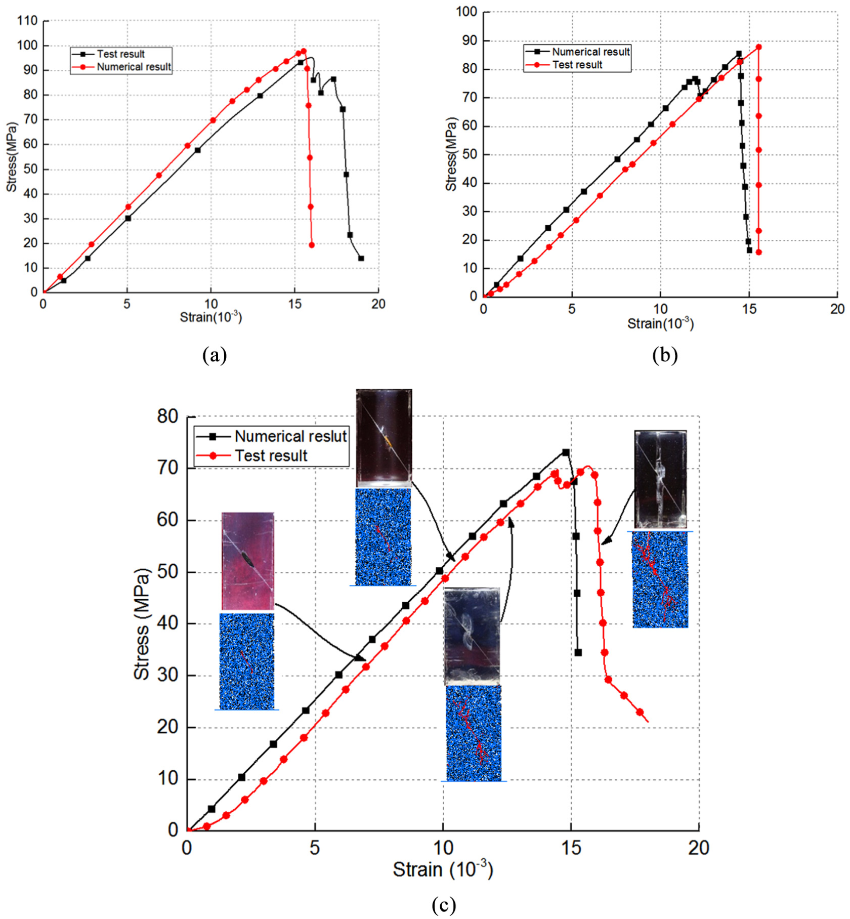
Stress–strain curve of numerical simulation and laboratory test: (a) stress–strain curve of the intact case; (b) stress-strain cure of specimen with 30° inclination angle; (c) failure mode comparison when inclination angle is 60°.

Numerical simulation results

Modeling of single-flaw with different inclination angles

Figure 11 shows the stress–strain curves of the specimens with single-flaw of different inclination angles (respectively, 15°, 30°, 45°, 60°, and 75°). As shown in Figure 11, when the inclination angle is 15°, the peak stress is 92.32 MPa. With the increase of the inclination angle, the peak stress decreases first and then increases. When the inclination angle is 45°, the peak stress is 64.78 MPa. It indicates that the peak stress is so low that specimens are easily destroyed when the angle is about 45°, which is consistent with the previous test results. The process of flaw propagation and coalescence during the uniaxial loading of the specimen at the inclination angle of 15° is shown in Figure 11(a)–(d). When the loading stress reaches about 40–50 MPa, the small flaws generate at two tips of the flaw. With the increase in stress, the small flaws around the flaw develop and coalesce into larger flaws, especially at two tips. Since then with the axial stress increases, flaws quickly extend to the upper and lower directions, which makes the flaw wing-shaped. At this point, the strength of the specimen is close to the limit strength. With the increase of load, the deformation is large but the stress is increased very small. When the strain reaches a certain value, the brittle specimen is damaged, and the stress drops quickly.

Figure 11.

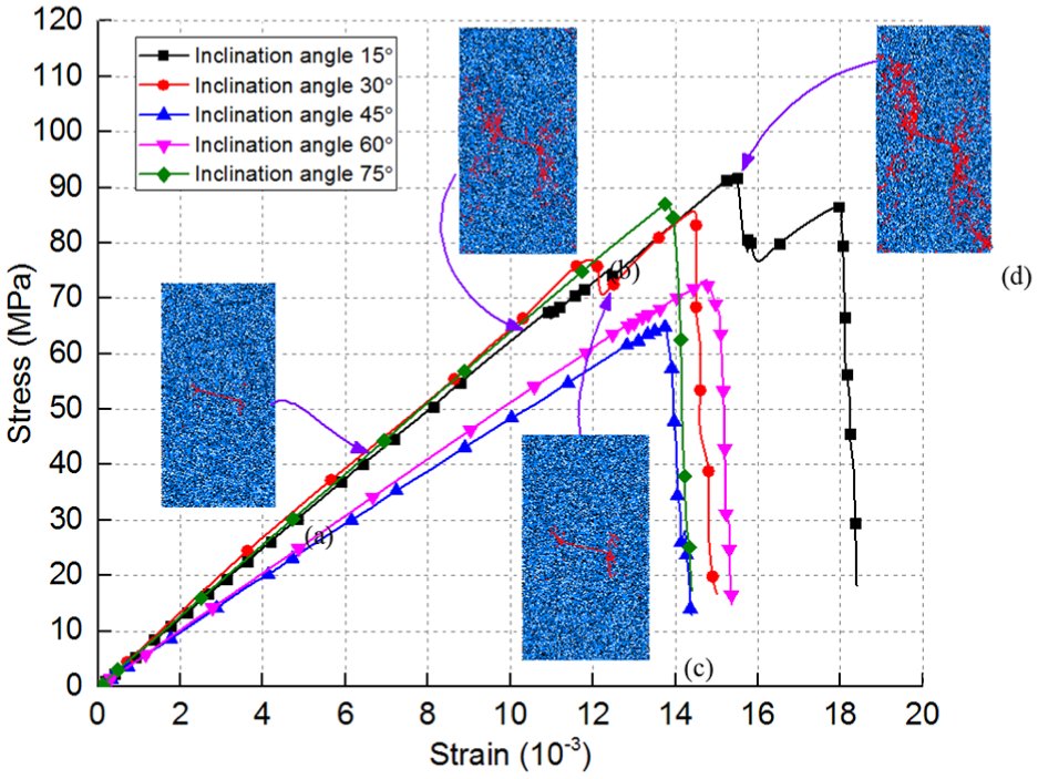
DEM with different flaw inclination under uniaxial compression, where (a) is the rock initiation stress at the inclination angle of 15°; (b) is the flaw propagation process and coalescence; (c) is the process of extension into the wing flaw; and (d) is the tension and splitting failure due to wing flaw extension.

Modeling of single-flaw with different lengths

Taking the specimen with 45° inclination angle as an example, the numerical simulation test of uniaxial compression was carried out while keeping other parameters unchanged. The flaw length was, respectively, 0 (intact specimen), 20, 40, and 50 mm. Figure 12 shows the stress–strain curves of the specimens with single-flaw of different lengths. It can be seen from Figure 12 that the peak strength of the intact specimen is 95.44 MPa. With the increase in the flaw length, the peak stress decreases gradually. When the flaw length is 50 mm, the peak stress is only 52.32 MPa.

Figure 12.

Strength and failure rules of different flaw lengths, where (a) is the final condition of 50 mm flaw length; (b) is the final condition of 40 mm flaw length; (c) is the case of 20 mm flaw length; and (d) is the length of 0 mm case.

It can be seen from the rose chart in Figure 12 that when the flaw length is 20 mm, the flaw with an inclination angle of 60°–120° accounts for 55.15% of the total. When the length of the flaw is 40 mm, the flaw with an inclination angle of 60°–120° accounts for 50.73% of the total. When the length is 50 mm and when the length of the flaw is 40 mm, the flaw with an inclination angle of 60°–120° accounts for 39.41% of the total. It indicates that the inclination angle of the flaw has a tendency to decrease with the increase in the flaw length. In general, the damage of the specimen is no longer caused by the longitudinal through crack, but it is caused by the fact that the wing flaws extend to the side and directly penetrate the side of the specimen.

Modeling of double-flaw with different spacing

According to Figure 13(b) and (c), the influence of double-flaw with different spacings on the failure pattern was studied. Figure 13 shows three different DEM models with different flaw spacings of 10, 20, and 30  mm. The two flaws are parallel to each other, and the connection line between the lowest point of the upper flaw and the highest point of the lower flaw is perpendicular to the flaws, and the center of the connection line is the center of the DEM model. With the single factor analysis method, other factors were kept unchanged to study the effect of flaw spacing on mechanical properties, where the inclination angle is 60°.

Figure 13.

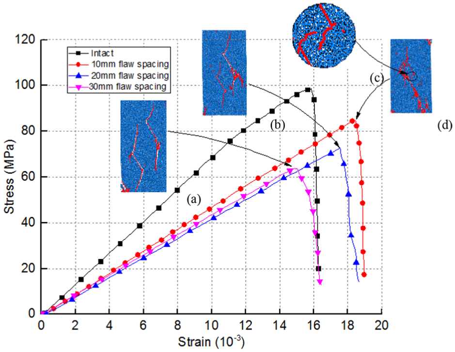
Effect of flaw spacing on failure mode under uniaxial compression: (a) peak stress condition of the sample. So as the (b) and (d). (c) Enlarged part of rock bridge.

When the flaw spacing is 30 mm, the main failure mode of the specimen is two relatively independent wing-shaped splitting tensile cracks, as shown in Figure 13(a). When the flaw spacing is 20 mm, the tips of upper flaw and lower flaw link each other. As shown in Figure 13(b), a rhombus-shaped damage zone is formed at the center of specimen. In the case of 10 mm flaw spacing, the upper flaw links the lower flaw and a rock bridge is formed as a vertical main fracture through the specimen, as shown in Figure 13(c) and (d).

Conclusion

In this article, in order to study the propagation and coalescence processes of pre-existing flaws in rock specimen, a series of uniaxial compression tests were carried out on built-in flaws of transparent rock-like specimens under different occurrence states, and the mechanism of flaw propagation was studied based on numerical simulation by flow code. The main conclusions are as follows:

1. A new sample preparation method for rock samples was proposed. The non-saturated polyester resin material was used to prepare transparent rock-like samples by the steps of blending, baking, and freezing. By this method, the mechanical properties of the prepared rock-like samples close to those of the actual rock sample, which provides a good way to study the flaw propagation.

2. Through the uniaxial compression experiments, it is concluded that the flaw dip, flaw area, and flaw friction coefficient have important influences on the mechanical properties of fractured rock under the condition of single-flaw. With the increase in the flaw dip, the peak stress of the specimen first decreases and then increases, while the inclination angle is 45°, the peak stress is lowest. The relationship between the peak stress and the fracture area is the second negative correlation, and the relationship between the peak stress and the fracture friction is basically linear. In the case of double-flaws, the spacing of the composite flaw has an important influence on the strength of the sample. With the increase of the flaw spacing, the strength of the sample gradually decreases, but the effect of flaw spacing on the elastic modulus and the flaw initiation stress of the specimen is not obvious.

3. The particle flow numerical method was used to verify the laboratory tests of fractured rock samples. The comparison shows that the numerical simulation results are in good agreement with the experimental results. On this basis, the effect of flaw length on the deformation and failure of the specimen was studied. It is concluded that with the increase in the flaw length, the strength of the sample gradually decreases and the inclination angle of the flaw has a tendency to decrease. The damage of the specimen is no longer caused by the longitudinal through crack, but is caused by the fact that the wing flaws extend to the side and directly penetrate the side of the specimen.