Sage Journals: Discover world-class research

Abstract

Turbulence-induced agglomeration of fine particles/droplets in aerosol is important in various industrial and natural processes. Despite abundant theoretical and numerical studies on turbulent collision kernels, convincing numerical methods for industry-scale applications are still lacking. In this work, we develop a mixed Eulerian–Lagrangian model for the modeling of turbulence-induced agglomeration of fine particles/droplets. As advantages over Sommerfeld’s model, the present model searches for real collision pairs based on a new mesh-independent method and uses appropriate turbulent collision kernels to calculate the collision frequencies. Benchmark simulations are carried out and compared with the results provided by the well-characterized experiment by Duru et al.

Keywords

Aerosol numerical simulation particles turbulent flow agglomeration

Introduction

Fine particle/droplet agglomeration in turbulent flows plays important roles in various industrial and natural processes, for example, cloud dynamics, pneumatic conveying, fluidized beds, particle separation in cyclones, mixing devices, and pollution control.^1–3 Early studies on this subject include research on the growth of droplets in turbulent clouds,⁴ the collision rate of inertial particles in dust separation cyclones,⁵ and the production of particles from the gas phase in turbulent flows.⁶

Simulations in particle collision in turbulent flows can be classified into the Eulerian–Eulerian two-fluid model and the Eulerian–Lagrangian particle trajectory model. Two-fluid model is efficient in computation. However, it is based on various hypotheses and cannot give the details about particle motion, inter-particle collisions, and interactions between gas and particles in different zones of the flow field. In contrast, the particle trajectory model needs fewer assumptions in the formulation of equations. Trajectories of a large number of real particles actually existing in the field are calculated and collision pairs are to be found from all the trajectories in a deterministic way, which lead to more precise results and more detailed information.

Direct numerical simulation (DNS) is most straightforward in Eulerian–Lagrangian approach and has been extensively used in the analysis of collisions in isotropic turbulent flows.^7–11 Sundaram and Collins studied the rate of inter-particle collisions by DNS of particles in turbulent flow. They found that particles with small Stokes numbers behave similar to those predicted by Saffman and Turner,⁴ while particles with very large Stokes numbers have collision frequencies similar to kinetic theory.⁵ For intermediate Stokes numbers, the collision behavior is complicated. Similar work has been done by Wang et al.¹⁰ and Zhou et al.¹¹ They studied the turbulent collision rate of monodisperse and bidisperse inertial particles. Due to complicated particle–turbulence interactions (e.g. differential sedimentation, turbulent acceleration, and preferential concentration), the collision kernels they obtained are only suitable for specific conditions. Meyer and Deglon¹² summarized these effects and reviewed the abundant results obtained by DNS method. However, DNS requires high resolution for flow calculation and large particle tracking number which lead to extremely high computational consumption. It is therefore not affordable for industrial applications.⁷

In order to improve the calculation efficiency, some stochastic collision models in Eulerian–Lagrangian approach have been developed.^2,13–17 The Monte Carlo (MC) sampling is widely used, which allows a subset of particles to be tracked. For instance, dealing with droplet collisions during spray process, O’Rourke² proposed a stochastic algorithm. Particles are considered distributed uniformly in a numerical mesh cell, and the search of collision partners is conducted by looping through all the parcels in the mesh cell. As a result, this method manifests serious mesh dependency. The turbulent effect on the collisions, which is an important issue under turbulent flow conditions, is also not discussed in this method. As a more reasonable modeling, fictitious collision partners are used by Oesterle and Petitjean,¹⁵ Berlemont et al.,¹⁴ Sommerfeld,¹⁶ and so on. Among them, Sommerfeld’s model has been widely used,¹⁸ in which when a collision occurs, a fictitious second particle is generated according to the local probability density functions of particle diameters and velocities. Then, the MC process is carried out to determine the collision result. As for the turbulent effect, the particle relative velocities are modified by correlating the fictitious particle velocities with the real particles. The relation between them is given as a function of particle Stokes numbers. Good agreement between validating cases and large eddy simulation (LES) results was found in a homogeneous isotropic turbulence flow.¹⁶ Similar work was also done by Berlemont et al.¹⁴ However, Sommerfeld’s model is only valid for inertial particles, but how to deal with fine particle collision in turbulent flow and how Brownian motion effect would be accounted for have not been discussed.

Although validation work has been done by comparing LES and DNS, it is still not for sure how well the models are adapted to the real application conditions.¹⁹ Very few of them are verified by experiments. The reason is that the collisions are extremely difficult to observe or measure. Nevertheless, some indirect information can be carefully measured to describe collision rates, for example, the growth rate of the mean particle diameter or the decay rate of particle number density (e.g. Duru et al.’s experiment²⁰).

In our previous work,²¹ we have established a new mesh-independent model using an adaptable control volume to search for real collision partners and calculate the collision probability. The model shows low computational expense and stable performance for complex engineering applications. In this article, we further improve the accuracy of the collision calculation by involving turbulent effects. Different from Sommerfeld’s method,¹⁸ we choose appropriate turbulent collision kernels for different flow regimes. Benchmark simulations are then performed to compare with the well-characterized experiment by Duru et al.²⁰

Mathematical model

Eulerian–Lagrangian approach is adopted to describe the gas-particle two-phase flow with four-way coupling. The key features of the mathematical model are as follows.

Gas phase

The gas phase is assumed incompressible and governed by Eulerian conservation equations. The re-normalization group (RNG) k − ε model²² is employed as seen in the appendix for its relative simplicity and robustness.

Particles

Particle rotation is neglected. The translational motion of a particle in the gas is governed by Newton’s law. The trajectory of a discrete particle is predicted by integrating the force balance on the particle, which is written in Lagrangian reference frame. The particle motion equation can be written as follows

\frac{\partial v}{\partial t} = F_{D} (u - v) + \frac{g (ρ_{p} - ρ)}{ρ_{p}} + F

(1)

where F is an additional acceleration force, for example, Brownian force. For very small particles, forces including virtual mass force, Basset history force, Saffman force, and Magnus force are negligible as analyzed in our previous work.²³ We have indicated that Brownian motion would lead to considerable collision for fine particles, as described by equation (9) in section “Collision kernels.”F_D( u − v ) is the drag force with v being the particle velocity and

F_{D} = \frac{18 μ}{ρ_{p} d_{p}^{2}} \frac{C_{D} R e_{p}}{24}

(2)

where µ, ρ_p, and d_p are the fluid dynamic viscosity, particle density, and particle diameter, respectively, with Re_p being the relative Reynolds number defined as

R e_{p} = \frac{ρ d_{p} | u - v |}{μ}

(3)

In (2), C_D is the drag coefficient defined as $C_{D} = α_{1} + α_{2} / {Re}_{p} + α_{3} / {Re}_{p}^{2}$ , where α₁, α₂, and α₃ are constants that apply to smooth spherical particles over several ranges of Re given by Morsi and Alexander.²⁴

Inter-particle collision

General form of collision model

A stochastic collision model is used to calculate the particle collision rate. The parcel-based approach is employed. Each parcel consists of n real particles of identical properties. The particles within a parcel are assumed to be uniformly distributed in the control volume V_c where the parcel is currently located. As discussed in our previous work,²¹ rather than the mesh cell volume V, we use a physically reliable volume V_pr as the control volume V_c. The collision volume V_pr is self-adjustable according to the local particle density. The method has been validated to be mesh independent and efficient.²¹

The collision frequency is then determined in analogy to the kinetic theory of gases, by the following equation

f_{c} = \frac{n π {(r_{1} + r_{2})}^{2} v_{rel}}{V_{c}} = n_{p} π {(r_{1} + r_{2})}^{2} v_{rel} = n_{p} K

(4)

where r₁ and r₂ are the radii of the particles, while v_rel is the relative velocity of the two particles. n_p = n/V_c is the particle number density in the respective control volume. K = π(r₁ + r₂)²v_rel is defined as the collision kernel.

The collision probability is an exponential function of the collision frequency and the Lagrangian time step and is calculated as follows

P_{c} = 1 - e^{- f_{c} Δ t}

(5)

The time step can be altered in the collision subroutine to ensure accuracy and stability of the calculation by limiting it to Δt < 0.05/f_c. This allows for at most one binary collision per time step, as derived by Sommerfeld.²⁵

Two uniform random numbers, range in [0, 1], are assigned to determine the collision outcome. A first uniform random number X is assigned only if X is smaller than P_c so that a collision can take place. A second uniform random number Y is assigned if a collision happens. For liquid aerosols, collisions between droplets can result in bouncing, coalescence, and fragmentation. If the value of the actual collision parameter, b, defined as (r₁+ r₂)Y^1/2 is smaller than the critical offset, b_crit, then

b_{crit} = (r_{1} + r_{2}) \sqrt{min (1.0, \frac{24 f}{We})}

(6)

where We is the collisional Weber number defined as $We = ρ v_{rel}^{2} \bar{D} / σ$ , and f is a function of the relative radius r₁/r₂, defined as $f (r_{1} + r_{2}) = (r_{1} / r_{2})^{3} - 2.4 (r_{1} / r_{2})^{2} + 2.7 (r_{1} / r_{2})$ , then a coalescence takes place; otherwise, a grazing collision occurs where all of the colliding particles maintain their original physical properties except that their velocities change. However, the model is most applicable for low-Weber-number collisions where collisions result in bouncing and coalescence. Above a Weber number of about 100, the outcome of collision could be shattering. Details refer to Qian and Law.²⁶ The new velocities based on the conservation of momentum and kinetic energy are given as

{v'}_{1} = \frac{m_{1} v_{1} + m_{2} v_{2}}{m_{1} + m_{2}} + \frac{m_{2} (v_{1} - v_{2})}{m_{1} + m_{2}} (\frac{b_{1} - b_{crit}}{r_{1} + r_{2} - b_{crit}})

(7)

{v'}_{2} = \frac{m_{1} v_{1} + m_{2} v_{2}}{m_{1} + m_{2}} + \frac{m_{1} (v_{2} - v_{1})}{m_{1} + m_{2}} (\frac{b_{1} - b_{crit}}{r_{1} + r_{2} - b_{crit}})

(8)

To simulate the turbulent effect on collision rate, a random walking model is used to tracking the parcels.

Collision kernels

According to the kinetic theory,⁵ the inter-particle collision rate depends on the particle relative velocity v_rel (seen in equation (4)). However, for fine particles in turbulent flow, Brownian coagulation and turbulence effect have to be considered such that v_rel should be modified. Different from Sommerfeld’s method, we replace the collision kernel K in equation (4) with some developed kernels to calculate the collision probability.

The kernel for Brownian motion–induced collision is given by Otto et al.²⁷

K_{br} = \frac{2 k_{b} T}{3 μ_{f}} (\frac{1}{r_{1}} + \frac{1}{r_{2}}) (r_{1} + r_{2})

(9)

where the Cunningham correction is taken to be one, which is justified for the particle size range considered in this study.

Abundant results about turbulent collision kernels have been presented. Basically, the particle collision behaviors in turbulent flow are related to their Stokes numbers, for example, St → 0, St → ∞, or in between. The particle Stokes number here is defined as St = τ_p/τ_k, where τ_p = 2ρr₂/9µ_f is the particle viscous relaxation time and $τ_{k} = 1 / 〈 Γ 〉$ is the Kolmogorov time scale.

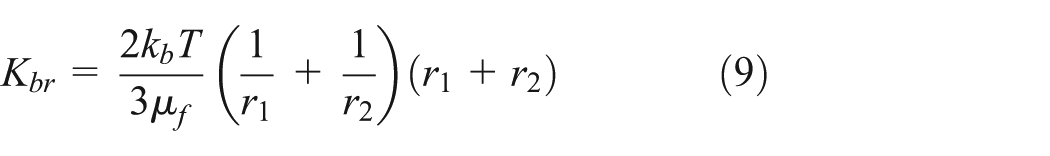
Saffman and Turner⁴ first derived the collision rate for particles with zero inertia in turbulent shear flow as

K_{s} = \sqrt{\frac{8 π}{15}} Γ {(r_{1} + r_{2})}^{3}

(10)

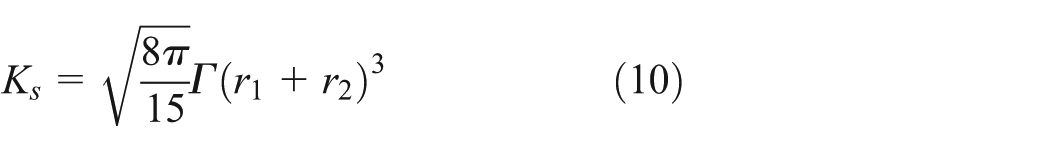
where r₁ and r₂ are the radii of the collision particles, and Γ is the Kolmogorov shear rate, which is related to the turbulent dissipation rate per unit mass ε and the fluid kinematic viscosity ν

Γ = {(\frac{ε}{ν})}^{1 / 2}

(11)

As discussed by Sundaram and Collins,⁸ particles with small Stokes numbers (St → 0) behave similar to the prediction of Saffman and Turner (equation (10)), and particles with very large Stokes numbers (St → ∞) have collision frequencies similar to kinetic theory, which is given by Abrahamson⁵

K^{\infty} = {(r_{1} + r_{2})}^{2} {(\frac{16 π {\bar{{v'}_{p}}}^{2}}{3})}^{1 / 2}

(12)

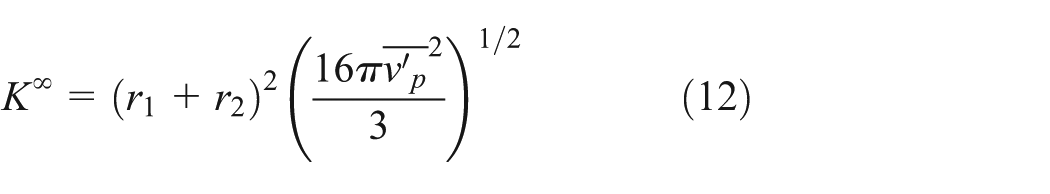
where $\bar{{v'}_{p}}$ is the variance of particle relative velocity, which is independent of turbulence properties.

For particles with intermediate Stokes numbers, both the turbulence and the particle mass play important roles and lead to complex collision behaviors, for example, preferential concentration, differential sedimentation, and other complex mechanism responsible for relative motion between particles.^8,12 Based on Saffman and Turner’s work, a modified kernel was analytically derived by Wang et al.¹⁰ with particle inertia and gravitational effects been included. Collision kernels have been intensively discussed through DNS. Sundaram and Collins⁸ investigated the influence of particle parameters such as response time, particle diameter, and number density on collision frequency in a monodisperse particle system. The exact expression for collision kernel was derived and verified based on the DNS database with Stokes number ranged from 0.4 to 8.0. Similarly, by including eddy-particle interaction, Zhou et al.¹¹ developed a bidisperse turbulent collision kernel (0.1 < St < 5.0). Wang et al.⁹ recently discussed the collision kernel (0.1 < St < 25) using a hybrid direct numerical simulation (HDNS) approach in which the effect of local hydrodynamic interactions of particles is considered. Some reviews on DNS works were summarized by Meyer and Deglon.¹²

The primary advantage of DNS is the accurate control of the flow and particle variables as well as the accurate collision statistics. However, the huge computational consumption places a severe restriction on the magnitude of Reynolds number and the Stokes number. Besides, their accuracy is still open to question since very few experiments are compared with.

In the presented model, the selection of appropriate kernel is decided by the particle Stokes number. For the St values in the reference experiment (as discussed in section “Particle mean radius growth”), the influence of preferential concentration on the collision rate is predicted to be only about 0.5%,²⁸ which means the inertial effect is small enough and therefore negligible. Therefore, Saffman–Turner kernel (equation (10)) could be used to describe the collision driven by turbulent shear. However, according to the recent experiment by Duru et al.,²⁰ the sedimentation and turbulent acceleration effects are comparable. A collision rate that accounts for gravity, turbulent shear, and turbulent acceleration, which was derived by Saffman and Turner and slightly corrected by Wang et al.,¹⁰ is also discussed in section “Results and discussions”

K_{t} = \sqrt{8 π} {(r_{1} + r_{2})}^{2} {[\frac{1}{15} Γ^{2} {(r_{1} + r_{2})}^{2} + {(1 - \frac{ρ_{f}}{ρ_{p}})}^{2} {τ_{p} (r_{1}) - τ_{p} (r_{2})}^{2} \times (1.3 g_{k}^{2} + \frac{π}{8} g^{2})]}^{1 / 2}

(13)

where g_k = ηΓ² is the turbulent acceleration experienced by particles much smaller than the Kolmogorov length scale. Turbulent acceleration and gravity-induced coalescence are absent among the drops of the same size so that K_t restores to K_s when r₁ = r₂.

On the other hand, according to the Kolmogorov shear rates Γ and initial particle radii in the experiment (Table 3), K_br/K_s is in the range 0.05–2, indicating that Brownian motion also plays a significant role. The collision kernel considering both Brownian and turbulent effect is therefore²⁹

K_{all}^{2} = K_{br}^{2} + K_{turb}^{2}

(14)

which is then employed in our simulation.

Numerical treatment

About experiment

Although extensive experiments have been performed on the Brownian coagulation of aerosols,^30,31 the experimental knowledge of aerosol coalescence due to turbulence is lacking. Such experiments require a precise characterization of the turbulent flow field; they also need accurate measurements of the change in the properties of aerosols with sufficiently high concentrations so that the coalescence rate is significant. In addition, measurements of aerosol coalescence on Earth are influenced by coupled effects of Brownian motion, turbulent shear and acceleration, and gravitational settling, making the experiment design difficult. Some attempts focused on measuring the coagulation rate of solid aerosol particles, in stirred tanks^32,33 or in a turbulent pipe flow.³⁴ In these studies, coagulation effects are observed by measuring the decay of the aerosol number density once the turbulent flow is initiated. Since the turbulent flow field was not measured in these experiments, it is necessary to use engineering correlations whose accuracy may not be enough to interpret the experimental results.

Quite different from the previous studies, recently Duru et al.²⁰ presented elaborate measurements of the coalescence rate in a well-characterized turbulent flow. As shown in Figure 1, they used an oscillating grid in a chamber to generate turbulence in a continuous mode of operation. Rather than the aerosol number density, rapid changes of the mean aerosol radius are measured using phase-Doppler anemometry, which has good temporal and drop size resolution. Furthermore, the Kolmogorov shear rate is determined from measurements of the root-mean-square fluctuating velocity and the integral length scale of the turbulent flow. We choose this elegant experiment to validate our modeling.

Figure 1.

Sketch of the experimental apparatus.²⁰

Numerical treatment

The numerical solution is obtained using the pressure-based finite-volume scheme. Software package FLUENT 6.3³⁵ enhanced with user-developed codes is employed. The SIMPLE algorithm is used for pressure–velocity coupling. The RNG k − ε model is used to calculate the turbulent flow field.

In the experiment, the grid moves only in z direction, which means x–y plane could be treated as periodic cells. Thus, a two-dimensional simulation is performed to reproduce the turbulent flow field to reduce the computational cost. As denoted by a dotted rectangle in Figure 1, one representative unit of size 2.5 cm × 25 cm in the chamber is selected as the computational domain. As shown in Figure 2(a), the computational domain is discretized into 8826 quadrilateral elements with an average size of 0.84 mm. A mesh-independence test shows that when the mesh is refined to 6250 elements or more, the deviations of the maximum velocity in the flow field are less than 5%. A symmetric boundary condition is set across the grid region to simplify the turbulent chamber of full scale. The simulation time step is set to be 0.004 s; the whole flow time is 100 s, identical to the experimental value.

Figure 2.

(a) Mesh setup, (b) distribution of the shear rate Γ, and (c) distribution of the instantaneous velocity vectors around the grid wire.

At the beginning, that is, t = 0 s, 5000 parcels with equal particle number per parcel are placed at a random position in the domain. All the parameters of particles and air (as shown in Table 1) are set according to the experiment. Stochastic particle tracking with random eddy lifetime is implemented with the discrete phase model, and particle continuous-phase interaction is enabled. The calculations of particle collision time step and inter-particle collision process are performed using self-written program in VC language, which is taken as user-defined function (UDF) embedded in the calculation of gas-particle two-phase flow.

Table 1.

Physical properties of the particles and air used in the simulations.

Properties	Particle (DEHS)	Air
Density (kg/m³)	916	1.205
Temperature (K)	293	293
Dynamic viscosity (kg/m s)	–	1.81 × 10⁻⁵
Kinematic viscosity (m²/s)	–	1.51 × 10⁻⁵
Surface tension (N/m)	3.2 × 10⁻²	–
Diameters (µm)	2.0–5.0	–
Number densities (×10⁵ particles/cm³)	1.5–26	–
Volume concentration (×10⁻⁶)	6.7–19.5	–

DEHS: di-ethyl-hexyl-sebacate.

The dynamic-mesh method is applied to describe the grid motion. As shown in Figure 2(a), the grid oscillating region, B, is same as the experimental parameter. The motion of the grid wire is set as sinusoidal motion to imitate periodic oscillation. Figure 2(c) shows a typical distribution of the instantaneous velocity vectors around the moving grid wire, while Figure 2(b) shows the distribution of the shear rate Γ at that moment. Different combinations of B and oscillation frequency f are used to produce different turbulent intensities. The values of the spatially and temporally averaged Kolmogorov shear rate $〈 Γ 〉$ obtained from experiments and simulations are listed in Table 2 for comparison. It is seen that all the simulation results are within the experimental measurement uncertainties, indicating that the simulations well reproduce the experimental turbulence.

Table 2.

The averaged Kolmogorov shear rate $〈 Γ 〉$ in experiments and simulations.

	$〈 Γ 〉_{Exp .}$ (s⁻¹)	$〈 Γ 〉_{Sim .}$ (s⁻¹)
B = 10 cm, f = 4 Hz	88 ± 11	94
B = 8 cm, f = 4 Hz	59 ± 9	63
B = 8 cm, f = 2 Hz	25 ± 3	28

Results and discussions

Particle mean radius growth

In the experiment, oil based (di-ethyl-hexyl-sebacate (DEHS)) aerosol is generated with nearly monodisperse. The aerosol number density n_i ranges from 1.5 × 10⁵ to 2.6 × 10⁶ particles/cm³. The aerosol mean radius r₀ ranges from 1 to 2.5 µm. The volume concentration is calculated to be in the range 6.7 × 10⁻⁶ to 19.5 × 10⁻⁶, and the Stokes number is therefore calculated to be in the range 3 × 10⁻⁴ to 6 × 10⁻³, which supports the use of Saffman–Turner kernel (as discussed in section “Collision kernels”).

There are 25 groups of experimental data, and all of them are used to compare the simulations. Table 3 shows three of them, where σ_r is the standard deviation of the fitting Gaussian distribution to the experimental particle size distribution. In the simulations, the temporal evolutions of the mean radius $〈 r 〉 (t)$ are measured. Figure 3 shows a typical plot of $〈 r 〉 (t) / r_{0}$ during the turbulent flow lasting for 100 s. The linear behavior of $〈 r 〉 / r_{0}$ is observed, which is similar to the experimental trend. Accordingly, the slope β of the fitting linear function is obtained.

Table 3.

Typical experimental conditions.

Exp. no.	r₀ (µm)	σ_r/r₀	No. of density (×10⁵ droplets/cm³)	$〈 Γ 〉$
1	1.45 ± 0.03	0.16	10	88
16	2.4 ± 0.06	0.18	1.5	59
25	1.87 ± 0.04	0.16	5.4	25

Figure 3.

A typical temporal evolution of $〈 r 〉 (t) / r_{0}$ from the beginning to the end of the simulation.

Comparison with experimental results

Simulation results are compared with the experimental results in Figures 4 –6. The Péclet number Pe is defined as: $Pe = 〈 Γ 〉 r_{0}^{2} / D_{B}$ where $D_{B} = k_{b} T / (6 π μ_{f} r_{0})$ is the Brownian diffusivity coefficient (k_b is the Boltzmann constant, T the temperature, and µ_f the gas viscosity). The error bars given for the experimental results (diamonds) are from the uncertainty in $〈 Γ 〉$ and in the measurement of the initial particle size distribution.

Figure 4.

β/n_i from simulation (squares) and experiment (diamonds), plotted as a function of Pe. Combination kernel includes K_br (equation (9)) and K_s (equation (10)).

Figure 5.

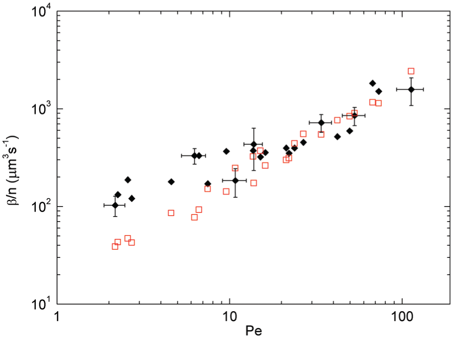
β/n_i from simulation (squares) and experiment (diamonds), plotted as a function of Pe. Kernel includes only K_s (equation (10)).

Figure 6.

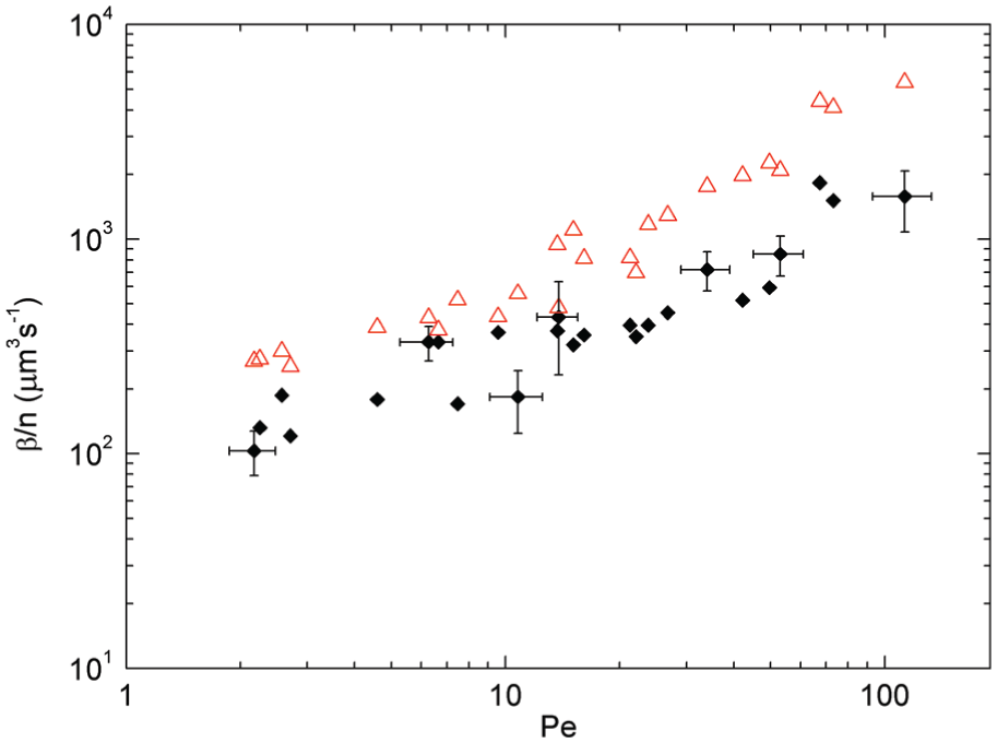
β/n_i from simulation (triangles) and experiment (diamonds), plotted as a function of Pe. Combination kernel includes K_br (equation (9)) and K_t (equation (13)).

Different combination kernels of K_br (equation (9)), K_s (equation (10)), and K_t (equation (13)) are used to conduct the simulation. Figure 4 shows the result of combination of K_br and K_s. It is seen that the simulation results are basically within the range of the experimental errors. Figure 5 shows the result of K_s alone. It is seen that when Pe < 10, the simulation results underestimate. According to the Kolmogorov shear rates Γ and initial particle radii in this range, we can find K_br/K_s > 0.5, indicating that Brownian motion starts to play a significant role. This result agrees with the experiment analysis by Okuyama et al.,³⁴ which verified that Brownian motion effect cannot be neglected when K_br/K_s > 0.1. Figure 6 shows the result of combination of K_br and K_t. The simulation result is 44% higher than the experiment result on average. The result is very close to Duru et al.’s theoretical result (40% overestimate when using K_t).

Besides the comparison of collision rate between the numerical and experimental results, the simulation reveals the details of the agglomeration process. For instance, Figure 7 shows typical particle size distributions obtained at the beginning and at the end of the agglomeration process. The decrease in the peak suggests that the agglomeration occurs and results in larger particles as time goes by.

Figure 7.

Typical particle size distribution obtained at the beginning and at the end of the simulation.

Conclusion

Although the turbulence-induced agglomeration of fine particle/droplet in aerosol is important in various practical fields, no convincing numerical methods have been available for modeling of industry-scale applications. In this article, we have developed a comprehensive mixed Eulerian–Lagrangian model. Different from Sommerfeld’s model,¹⁶ our model searches for real collision pairs based on a new mesh-independent model²¹ and uses appropriate turbulent collision kernels to calculate the collision frequencies. Benchmark simulations are carried out and compared with the results provided by the well-characterized experiment.²⁰ The simulation results are found in good agreement with the theoretical analysis by Duru et al.²⁰ Detailed information on the growth of particles mean diameter and the temporally evolving particle distribution is obtained.

Footnotes

Appendix 1

In the re-normalization group (RNG) k − ε model, the turbulence kinetic energy, k, and its rate of dissipation, ε, are obtained from the following transport equations

(15)

\begin{matrix} \frac{\partial (ρ k)}{\partial t} + \frac{\partial (ρ k u_{i})}{\partial x_{i}} = \frac{\partial}{\partial x_{j}} (α_{k} μ_{eff} \frac{\partial k}{\partial x_{j}}) \\ + G_{k} + G_{b} - ρ ε - Y_{M} + S_{k} \\ \frac{\partial (ρ ε)}{\partial t} + \frac{\partial (ρ ε u_{i})}{\partial x_{i}} = \frac{\partial}{\partial x_{j}} (α_{ε} μ_{eff} \frac{\partial ε}{\partial x_{j}}) \\ + C_{1 ε} \frac{ε}{k} (G_{k} + C_{3 ε} G_{b}) - C_{2 ε} ρ \frac{ε^{2}}{k} - R_{ε} + S_{ε} \end{matrix}

In these equations, G_k represents the generation of turbulence kinetic energy due to the mean velocity gradients. G_b is the generation of turbulence kinetic energy due to buoyancy. Y_M represents the contribution of the fluctuating dilatation in compressible turbulence to the overall dissipation rate. C_1ε, C_2ε, and C_3ε are constants. The quantities α_k and α_ε are the inverse effective Prandtl numbers for k and ε, respectively. S_k and S_ε are source terms. All the parameters are given by Chen.²²

Academic Editor: Takahiro Tsukahara

Declaration of conflicting interests

The author(s) declared no potential conflicts of interest with respect to the research, authorship, and/or publication of this article.

Funding

The author(s) disclosed receipt of the following financial support for the research, authorship, and/or publication of this article: This work is supported by the Natural Science Foundation of China (No. 91334110, No. 51276003) and Common Development Fund of Beijing.

References

Crowe

Schwarzkopf

Sommerfeld

. Multiphase flows with droplets and particles. Boca Raton, FL: CRC Press, 2011.

O’Rourke

. Collective drop effects on vaporizing liquid sprays. Princeton, NJ: Princeton University, 1981.

Tsotsas

Mujumdar

. Modern drying technology: vol. 1 computational tools at different scales. Dry Technol 2008; 26: 812–814.

Saffman

Turner

. On the collision of drops in turbulent clouds. J Fluid Mech 1956; 1: 16–30.

Abrahamson

. Collision rates of small particles in a vigorously turbulent fluid. Chem Eng Sci 1975; 30: 1371–1379.

Xiong

Pratsinis

. Gas phase production of particles in reactive turbulent flows. J Aerosol Sci 1991; 22: 637–655.

Mei

. On the collision rate of small particles in turbulent flows. J Fluid Mech 1999; 391: 67–89.

Sundaram

Collins

. Collision statistics in an isotropic particle-laden turbulent suspension. Part 1: direct numerical simulations. J Fluid Mech 1997; 335: 75–109.

Wang

L-P

Rosaa

Gaoa

. Turbulent collision of inertial particles: point-particle based, hybrid simulations and beyond. Int J Multiphas Flow 2009; 35: 854–867.

10.

Wang

L-P

Wexler

Zhou

. Statistical mechanical descriptions of turbulent coagulation. Phys Fluid 1998; 10: 2647.

11.

Zhou

Wexler

Wang

L-P

. Modelling turbulent collision of bidisperse inertial particles. J Fluid Mech 2001; 433: 77–104.

12.

Meyer

Deglon

. Particle collision modeling—a review. Miner Eng 2011; 24: 719–730.

13.

Anh Ho

Sommerfeld

. Modelling of micro-particle agglomeration in turbulent flows. Chem Eng Sci 2002; 57: 3073–3084.

14.

Berlemont

Chang

Gouesbet

. Particle Lagrangian tracking with hydrodynamic interactions and collisions. Flow Turbul Combust 1998; 60: 1–18.

15.

Oesterle

Petitjean

. Simulation of particle-to-particle interactions in gas solid flows. Int J Multiphas Flow 1993; 19: 199–211.

16.

Sommerfeld

. Validation of a stochastic Lagrangian modelling approach for inter-particle collisions in homogeneous isotropic turbulence. Int J Multiphas Flow 2001; 27: 1829–1858.

17.

Tanaka

Tsuji

. Numerical simulation of gas-solid two-phase flow in a vertical pipe: on the effect of inter-particle collision. In: 4th International symposium on gas-solid flows, vol. 121, Portland, 1991, pp.123–128. ASME FED.

18.

ANSYS, Inc. ANSYS 12.1 CFX-Solver Theory Guide, 2009, http://orange.engr.ucdavis.edu/Documentation12.1/121/CFX/xthry.pdf

19.

Hou

Schmidt

. Adaptive collision meshing and satellite droplet formation in spray simulations. Int J Multiphas Flow 2006; 32: 935–956.

20.

Duru

Koch

Cohen

. Experimental study of turbulence-induced coalescence in aerosols. Int J Multiphas Flow 2007; 33: 987–1005.

21.

Zhang

Wang

. A new mesh-independent model for droplet/particle collision. Aerosol Sci Tech 2012; 46: 622–630.

22.

Chen

. Comparison of different k-ε models for indoor air flow computations. Numer Heat Tr B Fund 1995; 28: 353–369.

23.

Zhang

Wang

. Fine particle behavior in the air flow past a triangular cylinder. Aerosol Sci Tech 2013; 47: 875–884.

24.

Morsi

Alexander

. An investigation of particle trajectories in two-phase flow systems. J Fluid Mech 1972; 55: 193–208.

25.

Sommerfeld

. Modellierung und numerische Berechnung von partikelbeladenen turbulenten Strömungen mit Hilfe des Euler: Lagrange-Verfahrens. Aachen: Shaker, 1996.

26.

Qian

Law

. Regimes of coalescence and separation in droplet collision. J Fluid Mech 1997; 331: 59–80.

27.

Otto

Fissan

Park

. The log-normal size distribution theory of Brownian aerosol coagulation for the entire particle size range. Part II: analytical solution using Dahneke’s coagulation kernel. J Aerosol Sci 1999; 30: 17–34.

28.

Chun

Koch

. Coagulation of monodisperse aerosol particles by isotropic turbulence. Phys Fluid 2005; 17: 027102.

29.

Zaichik

Solov’ev

. Collision and coagulation nuclei under conditions of Brownian and turbulent motion of aerosol particles. High Temp 2002; 40: 422–427.

30.

Abbott

. Experimental cloud droplet collection efficiencies. J Geophys Res 1974; 79: 3098–3100.

31.

Wagner

Kerker

. Brownian coagulation of aerosols in rarefied gases. J Chem Phys 1977; 66: 638.

32.

Langstroth

Gillespie

. Coagulation and surface losses in disperse systems in still and turbulent air. Can J Res 1947; 25: 455–471.

33.

Okuyama

Kousaka

Kida

. Turbulent coagulation of aerosols in a stirred tank. J Chem Eng Jpn 1977; 10: 142–147.

34.

Okuyama

Kousaka

Yoshida

. Turbulent coagulation of aerosols in a pipe flow. J Aerosol Sci 1978; 9: 399–410.

35.

FluentInc. Fluent 6.3 user’s guide, 2006, http://aerojet.engr.ucdavis.edu/fluenthelp/html/ug/main_pre.htm

An industry-scale modeling for the turbulence agglomeration of fine particles

Abstract

Keywords

Introduction

Mathematical model

Gas phase

Particles

Inter-particle collision

General form of collision model

Collision kernels

Numerical treatment

About experiment

Numerical treatment

Results and discussions

Particle mean radius growth

Comparison with experimental results

Conclusion

Footnotes

Appendix 1

Declaration of conflicting interests

Funding

References