
Abstract
The discrete solid element method is an efficient numerical method that simulates the large deformation, strong material nonlinearity, fracture, and dynamic problems of continuity. In the discrete solid element method model, the spring stiffness of the spherical elements on the boundary is different from that inside the discrete solid element method model based on the principle of conservation of energy. The spring stiffness of the spherical elements on the boundary of the discrete solid element method model is shown to have a significant effect on the macroscopic properties. According to the position of the spherical elements on the boundary of the discrete solid element method model, the spherical elements on the boundary are divided into three types, which are spherical elements on the surface position, on the edge position, and on the corner position. To accurately reflect the mechanical behavior of the material, the principle of energy conservation is used to strictly deduce the spring stiffness of the three types of spherical elements on the boundary, and the relationship between the spring stiffness and elastic constants is established. The numerical example shows that the calculation accuracy of the discrete solid element method in modeling the mechanical behavior of continuity is improved after the spring stiffness of the spherical elements on the boundary is revised. In addition, the applications of the discrete solid element method to dynamic buckling of the thin plate and buckling of the cracked thin plate are also given.
Keywords
Introduction
In the field of numerical calculation, the finite element method (FEM) is widely used to solve various mechanical and nonlinear problems due to its perfect theory and mature commercial software. The basis of the FEM is the variational principle and continuum mechanics. In terms of unit deformation solution, the FEM must satisfy the deformation coordination condition. Therefore, it’s difficult to simulate the strong nonlinear mechanical behavior of materials using the FEM, which requires special processing and complicated correction. Khoei et al. 1 used the arbitrary Lagrangian–Eulerian technique in the FEM to solve large deformation problems of solid mechanic. Lynn and Isobe 2 develop a FEM code that applied the adaptively shifted integration (ASI)–Guess technique to cope with strong non-linearity and discontinuity problems.
In order to overcome the shortcomings of the continuum mechanics method, the meshless method has been fully developed. The discrete element method (DEM) proposed by Cundall and Strack 3 is one of the representatives of the meshless method. In the DEM calculation process, the damping is used to dissipate energy so that the calculation converges. Qi and Ji-Hong 4 studied the calculation of damping force and the selection of damping coefficient. The Nonlinear viscous damping is used to calculate static problems. While for the dynamic problem, the selected damping should be able to reproduce the real response of the natural system under the dynamic load and the Rayleigh damping is used to calculate the dynamic problem.
In the DEM, the material is discretized into mass particles with the same or different sizes. The particles can move, touch, and collide in the analysis process of the DEM without a need to deliberately meet the deformation coordination and continuous condition. Therefore, the DEM is especially suitable for solving the large deformations and the strong nonlinear problems compared with the FEM. In recent years, DEM has been an effective numerical tool to solve the dynamic and fracture problems of the continuum.
Cheng et al. 5 introduced a two-dimensional (2D) discrete element model of hexagonal arrangement to solve the impact problem. A DEM model is proposed for the large deformation and strong nonlinear analysis of member structures by Ye and Qi, 6 and introduces the establishment and solution of the equations of motion and contact constitutive equations. Hentz et al. 7 used the DEM to model concrete subjected to dynamic loading at high strain rates. The cohesive beam model in the DEM was chosen by André et al. 8 and Meguro and Tagel-Din 9 to simulate the static and dynamic mechanical behavior of continuous materials. Griffiths and Mustoe 10 used a grillage of structural elements derived from the DEM concepts to simulate an elastic continuum. Sinaie 11 and Hentz et al. 12 applied the DEM to solve the fracture problem of concrete structures. These applications show that the DEM has been employed successfully in solving the elastoplastic, fracture, and dynamic and strong nonlinear problems of continuity.
FEM is not ideal for the simulation of large deformation problems, while the DEM is suitable for dealing with material damage and large deformation problems. For many problems in the structure, the region where the large deformation occurs is only a part of the material, and the material deformation is small in most regions. Therefore, the DEM simulation is applied to local and large deformation regions, and the other small deformation regions are simulated by FEM. The advantages of the two calculation methods are comprehensively combined, and the combined finite DEM is established. Munjiza et al. 13 and Rousseau et al. 14 developed a combined finite discrete element model for failure and collapse of reinforced concrete structure. Lei and Zhang 15 used an algorithm combining three-dimensional (3D) discrete and FEMs to simulate the impact fracture behavior of a laminated glass plate. Azevedo and Lemos 16 presented a DEM/FEM coupling algorithm which enables the use of rigid circular particles only on the fracture processes, the remaining part of the structure being modeled with finite elements.
For the nature of the random distribution of particles in soil and rocks, the random arrangement of spherical elements is suitable for simulating granular material. The DEM with the random arrangement of spherical elements was employed for simulating nonlinear mechanical behaviors, large deformations, strain softening, and dynamic fracture of soil grains and rock by Li et al., 17 Bono and McDowell, 18 and McDowell. 19 For the continuum problems addressed by the DEM, the regular arrangement of spherical elements is more suitable in terms of accuracy and efficiency compared with the random arrangement of spherical elements. The discrete solid element method (DSEM) with the cubic arrangement of spherical elements is proposed to calculate the extremely large deformation and strong material nonlinearity of continuity by Zhu and Feng. 20 The precision of the discrete gird is determined by the radius of the spherical elements. For the random arrangement, the radius of the spherical elements is determined by the size of the actual particles in the granular material. For the regular arrangement, the radius of the spherical elements is determined by the geometric size of the continuum structure.
In the DSEM, eight spherical elements constitute a DSEM cubic model. When the continuity is simulated by the cubic arrangement of spherical elements, the number of spherical elements connected to the spherical elements on the boundary of the DSEM model is different from that connected to the spherical elements inside the DSEM model, resulting in the spring stiffness of the spherical elements on the boundary being different from that inside the calculation model based on the principle of conservation of energy. If all the springs adopt the spring stiffness of the spherical elements inside the DSEM model, the displacement and the contact force of the spherical elements on the boundary will produce large errors. Especially in the case of controlling the number of spherical elements, when the DSEM is used to simulate the mechanical behavior of thin-walled structures, the displacement and the contact force of the spherical elements on the boundary may produce erroneous results.
The main purpose of this article is to derive the spring stiffness of the spherical elements on the boundary of the DSEM model using the principle of conservation of energy and to establish the relationship between the spring stiffness and elastic constants. Through revising the spring stiffness of the spherical elements on the boundary, the displacement and the contact force errors of the spherical elements on the boundary are reduced, and the accuracy of the simulation of the mechanical behavior of continuity obtained using the DSEM is improved. First, the physical model and the calculation principle of the DSEM are introduced, including the motion equation, elastoplastic force–displacement equations, and yield equation. Second, the spherical elements on the boundary are classified according to their positions, including the spherical elements on the surface position, on the edge position, and on the corner position. The principle of energy conservation is used to derive the spring stiffness of various spherical elements on the boundary. Finally, the spring stiffness of the spherical element on the boundary is verified by the thin plate example, with prominent boundary problems. Moreover, the ability of simulating strong nonlinear mechanical behaviors using the DSEM is demonstrated by the dynamic buckling of the thin plate and the buckling of the cracked thin plate.
DSEM
Physical model
In the DSEM, the material is discretized into mass spherical elements. As shown in Figure 1, eight spherical elements compose the basic cube model in the DSEM. The two spherical elements that are located on the edge and the diagonal line of the DSEM basic cube model are connected by springs. Therefore, there are two different groups of springs in the DSEM model, which are the springs on the edge and the diagonal line. Each group of springs includes one normal spring
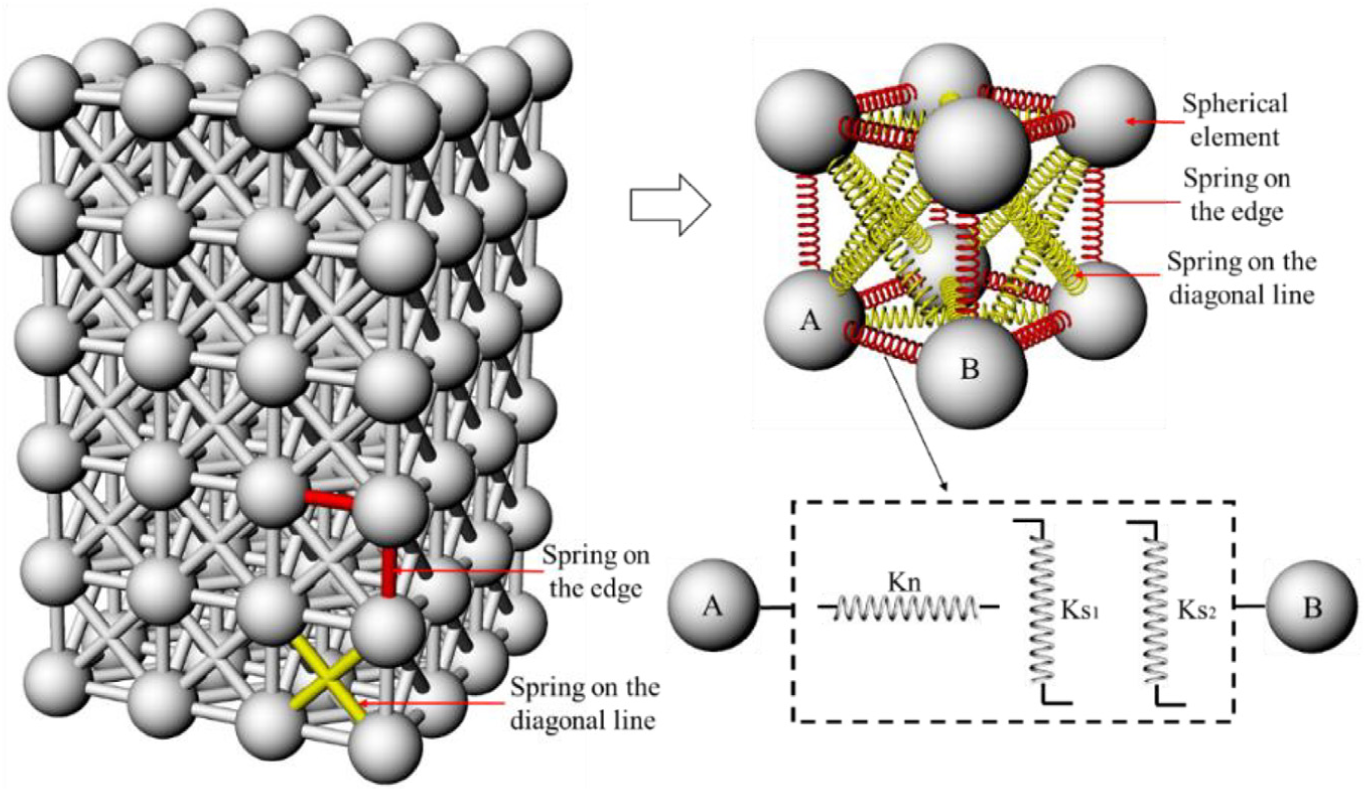
Physical model of DSEM.
Calculation principle
The main calculation flowchart of the DSEM is shown in Figure 2(a). The motion equation (Newton’s second law of motion) is applied to calculate the velocity and displacement of the spherical elements, and the force–displacement equation is applied to calculate the contact force (spring force) between spherical elements. The calculation flow is show in Figure 2(b). Given the relative displacement between spherical elements (obtained from the previous time step), the contact force between spherical elements is updated by the force–displacement equation. Then, according to the contact force and the motion equation, the velocity and displacement of the spherical elements are updated.

(a) Calculation cycle and (b) calculation flow.
The motion equation, as presented in equation (1), is solved by using the explicit central finite difference scheme. Then, the displacement of the spherical element i at
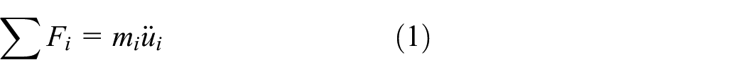

where
In the DSEM, the relationship between the contact force increment and the relative displacement between spherical elements is described by the force–displacement equation. The elastoplastic force–displacement equations for a perfect plastic material in the DSEM are presented in equation (3)

where
f is the yield equation in the DSEM, as presented in equation (4)

where
Spherical elements on the boundaryof the DSEM model
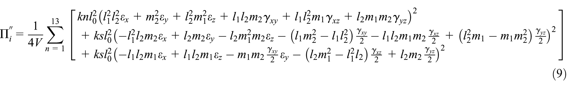
The spring stiffness of the spherical elements on the boundary has an important influence on the mechanical behavior of continuity modeled using the DSEM. As shown in Figure 3, according to the position of the spherical elements on the boundary of the DSEM model, the spherical elements on the boundary are divided into three types, which are the spherical elements on the surface position, on the edge position, and on the corner position. The number of the surrounding spherical elements connected to the spherical elements inside the DSEM model is different from that connected to the spherical elements on the boundary. The spherical elements inside the DSEM model are in contact with 18 surrounding spherical elements, as shown in Figure 4. The spherical elements on the surface of the boundary are in contact with 13 surrounding spherical elements, as shown in Figure 5. The spherical elements on the edge of the boundary are in contact with 9 surrounding spherical elements, as shown in Figure 6. The spherical elements on the corner of the boundary are in contact with 6 surrounding spherical elements, as shown in Figure 7. Therefore, the spring stiffness deduced from 18 spherical elements cannot be applied to spherical elements on the model boundary. The spring stiffness of the spherical elements on the boundary is different from that inside in the DSEM model based on the principle of conservation of energy. When the material is discretized into regularly arranged spherical elements in the DSEM, the spring stiffness of spherical elements on the boundary cannot adopt the spring stiffness of spherical elements inside the DSEM model. The spring stiffness of spherical elements on the boundary has an important influence on the macroscopic properties, the spring stiffness of spherical elements on the boundary need to be deduced to accurately simulate the mechanical behavior of the continuum boundary.

Spherical elements on boundary of DSEM model.

Spherical element inside model contact with 18 surrounding spherical elements.

Spherical element on surface of boundary contact with 13 surrounding spherical elements.
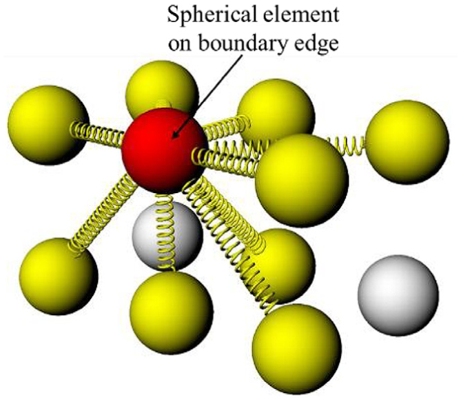
Spherical element on edge of boundary contact with 9 surrounding spherical elements.

Spherical element on edge of boundary contact with 6 surrounding spherical elements.
Spring stiffness deduction of spherical elements on the surface
In the DSEM, the spherical elements and springs form a network system that captures the complicated mechanical behavior of continuity. To accurately reflect the mechanical response of the material, the spring stiffness in the force–displacement equation is critical. The relationship between the spring stiffness and the elastic Modulus E and Poisson’s ratio

where

Spherical element on surface of boundary.
The relative displacements between spherical elements can be expressed by the strain and the central distance, as presented in equation (6)

where
The transformation matrix is given by

where
Thus, the strain in the local coordinate system can be written in terms of global strain quantities by transformation equations, as presented in equation (8)

where
Substituting equations (6) and (9) into equation (5) yields
Assume that the radius of a spherical element is r and that the initial central distances of two spherical elements on the edge and the diagonal line of the model are


Contact force on one spherical element on surface of boundary.
According to the elastic mechanics used by Xu, 21 the strain energy density can be expressed as

The strain energy densities expressed by equations (10) and (11) are equivalent, and the following assumptions of Jefferson et al.
22
are used:
Solving equation (12), the spring stiffness of a spherical element on boundary surface is given by

Spring stiffness deduction of spherical elements on the edge
As shown in Figure 10, the spherical element on the edge of boundary is connected with nine surrounding spherical elements. There are four surrounding spherical elements with the initial central distance of
The spring stiffness of a spherical element on boundary edge is given by


Spherical element on edge of boundary.

Contact force on one spherical element on edge of boundary.
Spring stiffness deduction of spherical elements on the corner
As shown in Figure 12, the spherical element on the corner of boundary is connected with six surrounding spherical elements. There are three surrounding spherical elements with the initial central distance of
The spring stiffness of the spherical element on the boundary corner is given by

Spherical element on corner of boundary.

Contact force on one spherical element on corner of boundary.
Numerical examples
Elastoplastic bending of thin plate
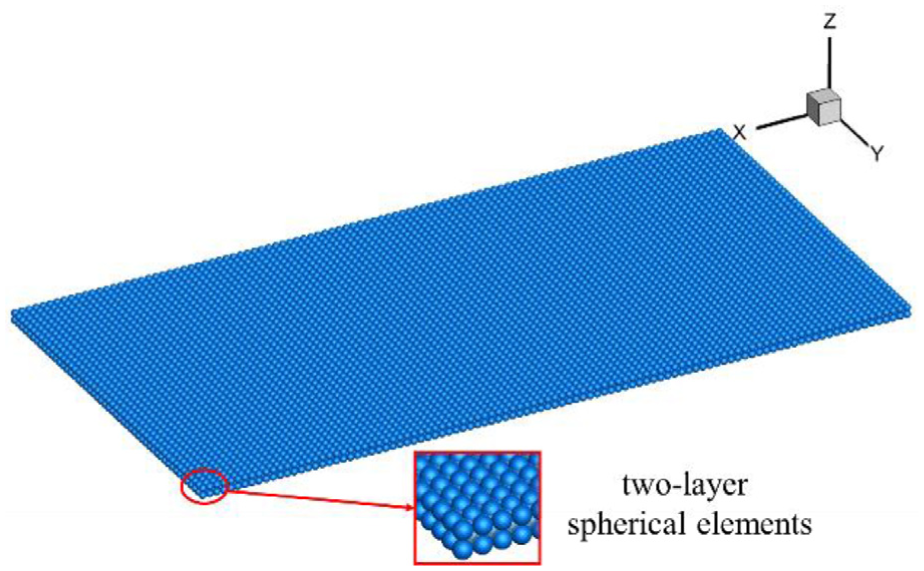
In this example, the elastoplastic bending of a thin plate subjected to uniformly distributed loads is simulated. The purpose is to study the effect of the spring stiffness of the spherical elements on the boundary on the mechanical behavior of continuity modeled using the DSEM. The FEM solution is used as the reference for evaluating the DSEM results. The geometry information, boundary conditions, and material properties are shown in Figure 14. The geometric dimensions of the thin plate are

Material parameters for elastic-plastic bending of thin plates.

DSEM model for elastoplastic bending of thin plate.

FEM model.
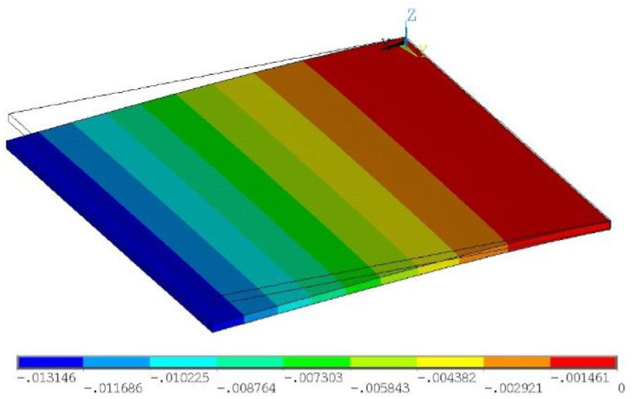
The simulation results of the FEM and the DSEM are shown in Figures 17 –24. The DSEM model can reproduce the same displacement and plastic distribution as the FEM model. This outcome means that the DSEM can be regarded as a valid representation of an isotropic elastoplastic material. To quantitatively study the calculation accuracy of the mechanical behavior of continuity simulated using the DSEM after revising the spring stiffness of the spherical elements on the boundary, two lines, Line I

X-direction displacement via FEM.

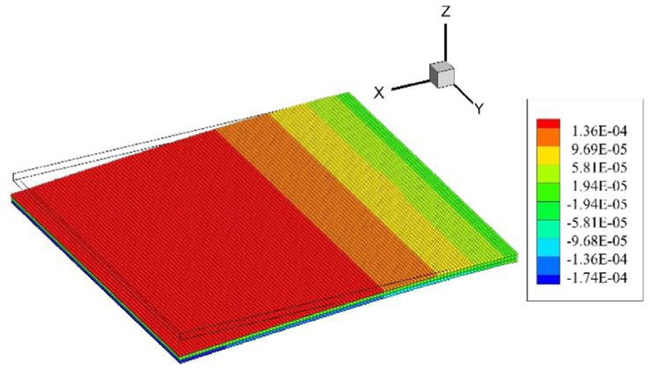
Y-direction displacement via FEM.
Z-direction displacement via FEM.

Plastic distribution via FEM.
X-direction displacement via DSEM.

Y-direction displacement via DSEM.
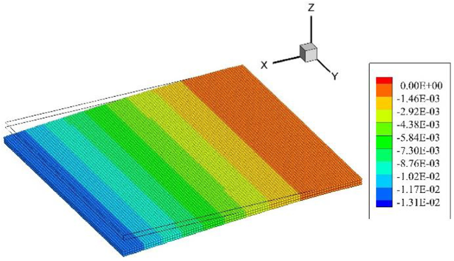
Z-direction displacement via DSEM.

Plastic distribution via DSEM.
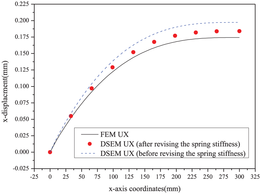
Comparison of x-direction displacement of Line I.
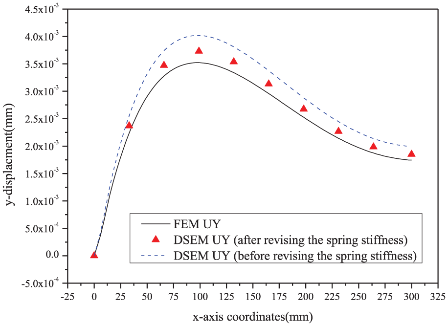
Comparison of y-direction displacement of Line I.
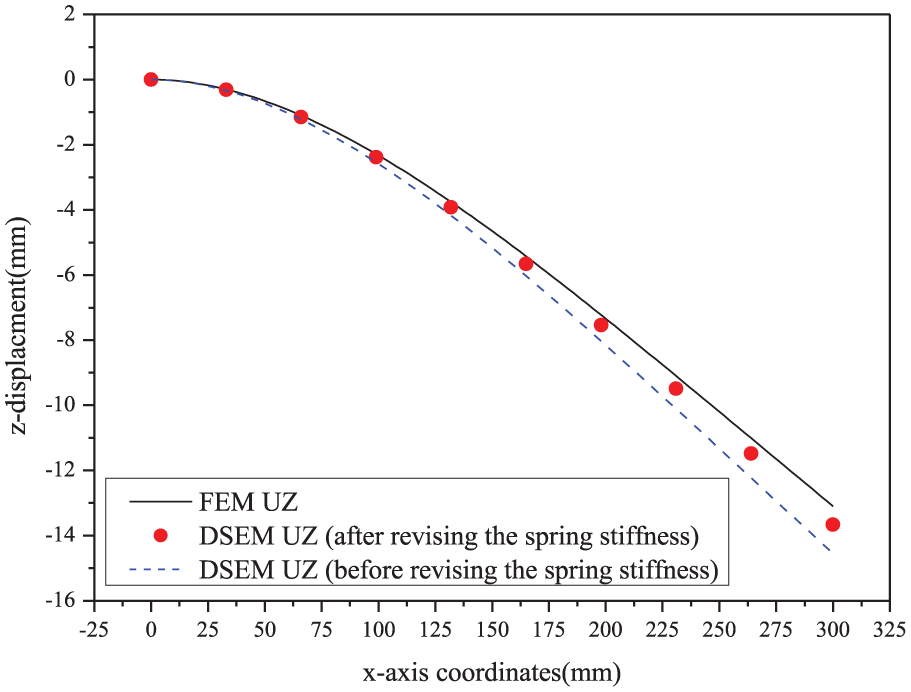
Comparison of z-direction displacement of Line I.

Comparison of x-direction displacement of Line II.

Comparison of y-direction displacement of Line II.
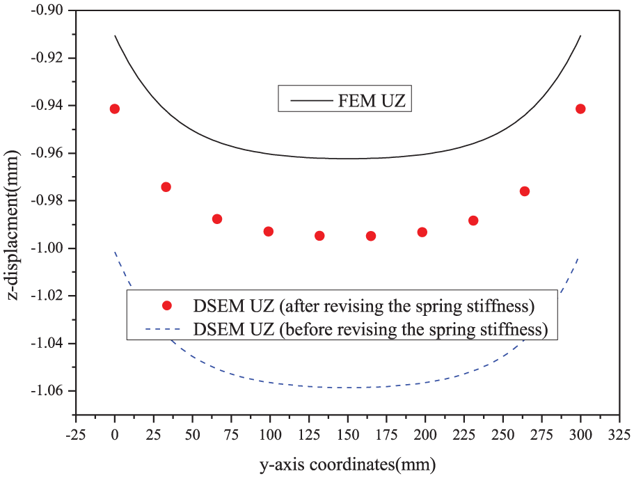
Comparison of z-direction displacement of Line II.
The concept of a contact force between the spherical elements in the DSEM is different from the stress concept in traditional mechanical theory. Therefore, the internal force is selected for comparison. The thin plate is only subject to the uniform load in the z-direction; thus, the internal force in the x- and y-directions is approximately
Results of the internal force in the z-direction.

FEM: finite element method; DEM: discrete element method.
Dynamic buckling of thin plate
In this section, the DSEM is used to simulate the dynamic buckling of a thin plate. The purpose of this approach is to show the potential of the DSEM when solving the extremely large deformation and high material nonlinearity problems of continuity. The experimental results by So and Chen
23
are used as the reference for evaluating the DSEM results. The geometry information, boundary conditions, and material properties are specified in Figure 31. The length of the thin plate is

Material parameters for dynamic buckling of thin plate.
DSEM model for dynamic buckling of thin plate.
Figures 33–35 show the front and side views of the typical deformation of the dynamic buckling of the thin plate obtained using the DSEM when the calculation times are

Deformation of thin plate when

Deformation of thin plate when

Deformation of thin plate when
Figure 36 shows the curve of the load against axial displacement for the loading end of the thin plate. When the axial load is applied, a series of peak loads of decreasing intensity are recorded during the progressive buckling of the thin plate. Through revising the spring stiffness of the spherical element on the boundary, the initial stiffness, the peak loads, and the corresponding displacement generated using the DSEM model more closely match the experimental results. After revising the spring stiffness, the first critical buckling load generated using the DSEM model decreases from

Variation of load versus displacement histories.

Variation of displacement versus time histories.
Buckling of cracked thin plate
In this section, the DSEM is used to simulate the buckling of a cracked thin plate. The purpose of this approach is to show the ability of the DSEM when solving the fracture problems of continuity. The experimental results by Seifi and Kabiri
24
are used as the reference for evaluating the DSEM results. The geometry information, boundary conditions, and material properties are specified in Figure 38. The thin plate has dimensions of
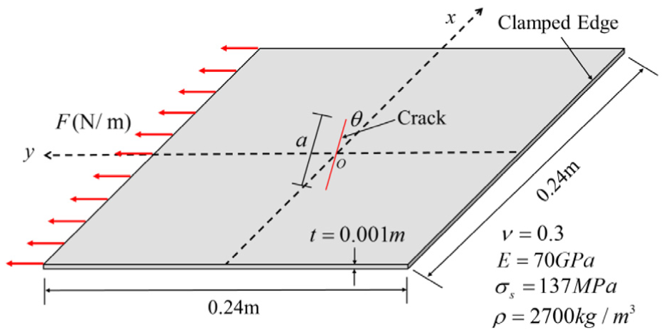
Material parameters for buckling of cracked thin plate.
Two cases are studied, as shown in Figure 39. The crack length is

Configurations of samples.

DSEM model for buckling of cracked thin plate.
The buckling forms of the thin plates are depicted in Figure 41. The buckling shapes in the tension correspond to the instability phenomenon with diffuse out-of-plane displacements localized around the cracked area. The DSEM results agree well with the experimental results of Seifi and Kabiri.
24
The comparison of the buckling load of the cracked thin plate is depicted in Table 2. Through revising the spring stiffness of the spherical elements on the boundary, the buckling load is reduced from

Buckling form by DSEM.
Comparison of the buckling load.
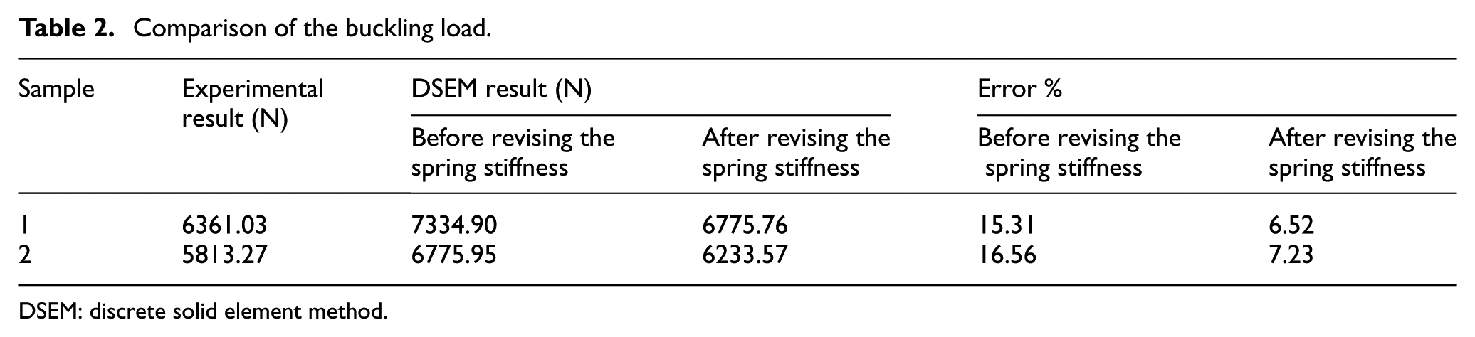
DSEM: discrete solid element method.
Conclusion
The DEM has been developed as a general and effective numerical calculation method for simulating the mechanical behavior of solid and granular materials, including the transformation from a continuum to a discontinuum. Because the mechanical behavior of the structure is calculated using the discrete grid system composed of spherical elements and springs in the DSEM, the spring stiffness has an important influence on the mechanical behavior of the structure. The spring stiffness of the spherical elements inside the DSEM model is different from that on the boundary when the continuity is modeled using the DSEM. In this article, the spring stiffness of the spherical elements on the boundary is deduced. The spring stiffness is verified using three examples. Through revising the spring stiffness of the spherical elements on the boundary, the displacement and contact force errors of the DSEM model are reduced effectively, and the calculation accuracy of continuity simulated using the DSEM is improved. In addition, through the simulation of dynamic buckling of a thin plate and the buckling of a cracked thin plate, the ability of the DSEM to address strong nonlinear, dynamic, and fracture problems is demonstrated. The following conclusions can be obtained:
According to the different positions of the spherical elements on the boundary of the DSEM model, the spherical elements on the boundary are divided into three types, which are spherical elements on the surface, on the edge, and on the corner. Based on the principle of energy conservation, the spring stiffnesses of the three types of spherical elements on the boundary are deduced.
The elastoplastic bending of a thin plate with a prominent boundary problem is simulated using the DSEM. In the DSEM model, the number of spherical elements on the boundary accounts for 67% of all spherical elements. Through revising the spring stiffness of the spherical elements on the boundary, the maximum displacement error in the x-direction decreases from 12.92% to 5.23%, the maximum displacement error in the y-direction decreases from 14.41% to 5.76%, and the maximum displacement error in the z-direction decreases from 11.38% to 4.31%. The maximum error of the internal force of the DSEM model is reduced from 3.81% to 1.64%.
The example of dynamic buckling of a thin plate subjected to compression shows that the DSEM can effectively solve the strong nonlinear and dynamic problems accompanied by multiple layers of wrinkles. After revising the spring stiffness of the spherical elements on the boundary, the error of the first critical buckling load decreases from 14.58% to 4.2% compared with the experimental results.
The example of the buckling of a cracked thin plate subjected to tension shows that the DSEM can effectively address fracture problems. Through revising the spring stiffness of the spherical elements on the boundary, the buckling load errors of a cracked thin plate decrease from 15.31% to 6.52% and from 16.56% to 7.23% in the first and second samples, respectively.
Footnotes
Handling Editor: Vesna Spasojević Brkić
Declaration of conflicting interests
The author(s) declared no potential conflicts of interest with respect to the research, authorship, and/or publication of this article.
Funding
The author(s) disclosed receipt of the following financial support for the research, authorship, and/or publication of this article: This research was financially supported by the Fundamental Research Funds for the Central Universities, by the Colleges and Universities in Jiangsu Province Plans to Graduate Research and Innovation (KYLX15_0089), by a project funded by the Priority Academic Program Development of the Jiangsu Higher Education Institutions, and the Natural Science Foundation of China under grant number 51538002.