
Abstract
As for the fact that the majority of current researches take the technology of tool-path planning for free-form surface only as a geometrical problem, which is not suitable for belt grinding because of the elastic deformation of the grinding belt that leads to a variable contact, in this article, the tool-path planning method for belt grinding is developed from the elastic contact point of view. Based on the Hertzian contact theory and taking the grinding force into consideration, a calculation method of the contact area between the belt and the workpiece is presented. Then, a tool-path planning model is presented based on the real contact area to meet the full coverage. In addition, an optimization model based on the constant scallop-height is further developed to meet the high form accuracy of the workpiece. First, a modified model for the material removal depth is developed based on the Preston equation. Then, according to the curvature of the contact surface, three situations are analyzed and the calculation methods of the tool-path interval are given. Finally, experiments on the simulation blade are conducted, and the experimental results show the effectiveness of the method in this article.
Introduction
With the ever-increasing requirements for manufacturing automation in the modern manufacturing industry, as the core part of digital design and manufacturing technology, numerical control (NC) programming for free-form surface becomes more and more important.1,2 And, as the basis of NC programming, tool-path planning has a very important influence on the manufacturing efficiency and quality of the workpiece, which makes it a key research content and an ever-increasing concern in industries and academia nowadays.3,4
As a hot and difficult topic in manufacturing field, tool-path planning for free-form surface is concerned with lots of key technologies such as the selection of cutting tools, processing interval, and interference detection. 5 The current studies focus on the determination of processing interval because of its significant impact on the manufacturing efficiency and quality.6,7 A large interval can easily lead to an unprocessed region between adjacent paths, and additional path is required, which will cost manufacturing time and decrease efficiency. While a small interval results in overlapping between adjacent paths. Overlapping may degrade the surface quality and decrease cutting-tool life as the same area is covered more than once. The two kinds of situations both result in increased manufacturing time and costs.
Therefore, many scholars have done extensive researches on the determination of the processing interval and achieved certain results. Elber and Cohen 8 developed an adaptive iso-curve extraction method to overcome the shortcomings of the parametric method. The method is utilized to decide whether to insert the sub-path by determining the distance between two adjacent tool-paths. Ding et al. 9 proposed an adaptive iso-planar method which is applied to partition the surface into different regions, and in each region, the tool-path intervals are adaptive to the surface features. Therefore, redundant tool-paths are avoided. Wu et al. 10 presented a method for determining the machining strip width of the flat-end cutter. This method depends on the intersection points between the effective cutting shape and the offset curve of the normal transversal along the path interval direction on the machined surface. Wang et al. 11 present a comprehensive tool-path generation strategy for slow tool servo (STS) turning of complex surfaces, including cutting point optimized planning, trajectory interpolation and machining simulation. Lo 12 and Lee 13 established a path planning method based on the geodesic line. In this model, the inclination angle can be chosen as small as possible so that a large path interval can be utilized to improve the machining efficiency.
Most of the above papers are conducted from the geometric perspective. While in belt grinding, in addition to geometric constraints, elastic deformation due to the low stiffness of the belt also has an important impact on path planning. 14 Especially for the workpiece with a large surface curvature, a simple geometrical method is more likely to lead to a large or small interval, which will reduce processing efficiency and quality. For the problem of path planning under elastic contact, Rososhansky and colleagues15,16 applied contact mechanics to model and analyze the actual contact area between the flexible polishing tool and the workpiece, then a contact area map was established and used to plan polishing paths that ensures a complete coverage. This method does not optimize the grinding quality by considering the removal depth. Roswell et al. 17 showed that the same polishing force may lead to different removal depths because of the varied workpiece curvature, which can affect the surface uniformity. Then, Cheng further considered the material removal and constructed a material removal function with correction weight. On this basis, the optimal tool-path was given under the constraint of minimum residual error. 18 Tian took the elastic sponge disk as the polishing tool and constructed the quadratic function as the material removal profile. Then, taking the consistent scallop-height of material removal as the constraint, the path planning method was presented. 19 All these studies provide a good guide for the path planning in the case of elastic contact.
Based on the above research works, in order to further reveal the actual elastic contact deformation of flexible grinding and optimize the grinding path under the quality constraint, a tool-path planning method for free-form surface in belt grinding is developed considering the elastic contact situation in this article. The full coverage model of the tool-path planning is presented based on the contact area between the belt and the workpiece in the “The full coverage model” section. Section “The optimization model of tool-path planning” presents a modified model of the material removal depth, and further, an optimization model based on the constant scallop-height is put forward to meet the requirement of high form accuracy. Experiments are conducted and the results are discussed in the “Experiments and discussion” section. The last section concludes with summary of major contributions from this work.
The full coverage model
During the process of belt grinding, the grinding belt suffers from the elastic deformation due to the grinding force, and the contact area between the belt and the workpiece will change, which has a great effect on the determination of the interval. Therefore, in this part, first, Hertzian contact theory is utilized to develop a model for the real contact area. And then, based on the area model, a full coverage model of the tool-path planning for free-form surface is presented.
The model of the real contact area
In this research, the grinding tool is a belt and the workpiece is a free-form surface with a definite elasticity. The contact between them obeys the Hertzian contact theory, namely: 20
The grinding belt and the workpiece are elastic and both experience small strains;
The dimensions of the deformed contact area remain small compared to the principal radius of the undeformed surface;
The contact surfaces are continuous prior to deformation.
Therefore, according to Hertzian contact theory, the contact area between the grinding belt and the workpiece is an ellipse and the boundary line of the elliptic area can be given by 21

where a and b are the semi-major axis and the semi-minor axis, respectively. Then, a and b can be calculated as follows 21


where F is the applied force between the belt and the workpiece surface;


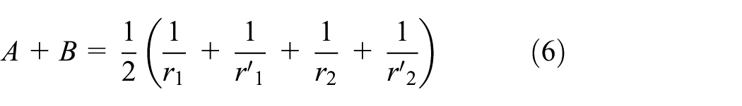

where
As we can see from equations (1)–(7), if all parameters are held fixed (i.e. grinding force, modulus of elasticity, and Poisson’s ratio), the contact area is just a function of one variable: the radius of curvature of the workpiece.
The full coverage model
As we see from the schematic diagram of the grinding path, as shown in Figure 1, it is a set of all discontinued paths along the workpiece surface and every path is a collection of distinct contact points. Known from above, every contact point implies a contact elliptic area which is a function of the curvature radius of the workpiece. Therefore, the grinding path is a set of ellipses. Note that the contact points are placed farther away from each other so that the contact areas will be more visual. In practice, however, the ellipse is much denser between contact points.

Schematic diagram of the grinding paths.
In Figure 1, Li represents the ith grinding path along the workpiece surface and Pik stands for the kth contact ellipse on path Li. Therefore, a single grinding path can be expressed as

where Pim represents the last contact ellipse on path Li. Then, the set of all paths can be presented as

where TP stands for the set of all paths and Ln is the last grinding path on the workpiece surface. Substituting equation (8) into equation (9) results in
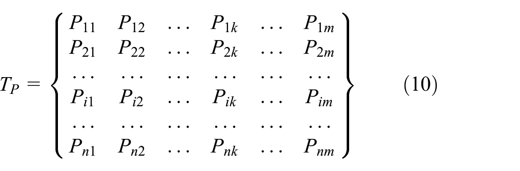
The interval between paths Li and Li + 1 is the distance between the center points Oi and Oi + 1 of the corresponding two contact ellipses. If their edges are connected with no gap or overlap, then this means a full and even coverage. Since the distance between ellipses depends only on the semi-major axis a and the semi-minor axis b has no effect, equation (10) can be changed into another form in terms of the semi-major axis a

According to equation (11) and under the requirement of a full and even coverage, the interval between paths Li and Li + 1 can be given by

where li is the interval between paths Li and Li + 1. Two situations are as follows:
The workpiece is a flat surface and then the radius of curvature is constant and approaches infinity. Therefore, the semi-major axis a will not change, which means that the interval between two paths is a constant;
The workpiece is a free-form surface and we can know the semi-major axis a changes with the radius of curvature. In this situation, the interval between two paths is a variable.
In the two situations, both a can be calculated by Hertzian contact theory. The detailed coordinates of grinding points are the basis of NC programming. Therefore, here is the method to calculate the coordinates of the contact points (the center points of the contact ellipses). In this article, it is assumed that Y-axis represents the grinding path direction and X-axis is the direction of the semi-major axis a. The determination of the coordinates along the Y-axis direction belongs to the research of processing step, and it is not discussed here. And, based on the analysis above, here, the method to calculate the coordinates along the X-axis direction is presented as follows. The coordinates for each contact point of a grinding path can be given by

where qik represents the coordinate of the kth contact point on the ith path along the X-axis direction. And then, the coordinate of the kth contact point on the (i + 1)th path can be calculated as follows

Based on the recursive equation (14), the coordinates along the X-axis direction of all the contact points can be calculated by matrix equation (15), and a full and even coverage will be achieved by adopting this matrix

The optimization model of tool-path planning
As for some high-quality-required workpiece, such as the aero-engine blade, only the full coverage of the grinding paths is not enough. In this part, by taking the form accuracy of the workpiece into account, an optimization model taking the scallop-height as the constraint is established based on the modified model of material removal depth.
The modified model of the material removal depth
In order to achieve the required form accuracy, a critical and difficult problem is to precisely control the removal of the material, namely, the quantitative removal of material. Therefore, it is necessary to develop a model of the material removal depth. Currently, the most commonly used method is based on Preston equation as shown in equation (16),22,23 which defines the material removal depth per unit time is proportional to the instantaneous velocity and pressure. And, the effect of other factors (such as processing materials and grinding tool) is considered to be a proportional constant K. In other words, Preston equation creates a linear relationship between the material removal depth and pressure, as well as instantaneous velocity

where h represents the removal depth, p is the pressure, and v stands for the relative velocity between the belt and the workpiece. Here are the methods to calculate the parameters in Preston equation for belt grinding.
The rotation speed of the belt and the feed speed of the workpiece are defined by vt and vf, respectively. And, v can be calculated as follows

When the direction of the feed rate is the same as that of the tool rotation, “–” is chosen, else “+” is chosen. The pressure distribution equation is as follows 21
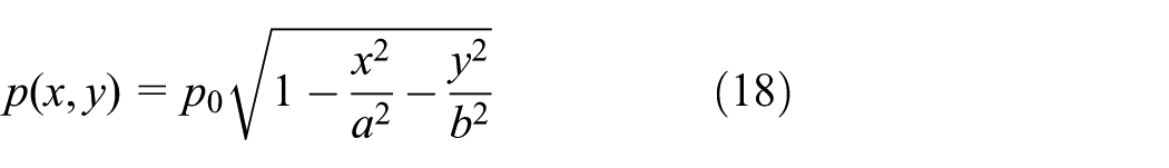
where a and b are the semi-major and semi-minor axes, respectively, which can be obtained by equations (2) and (3); p0 is the maximum contact pressure located at the center of the contact ellipse which can be given by 21

Substituting equations (17)–(19) into equation (16), the total removal depth of the contact point can be obtained by integrating equation (16). While as equation (18) shows, the pressure p is a function of the contact place, which makes it hard to establish a relationship with the grinding time, so the integration of equation (16) is difficult to obtain. Therefore, in this part, a modified model based on the original Preston equation is derived.
There exits an infinitesimal M of the workpiece surface in the contact region. It is assumed that during the time dt, the feed length of M in the contact region is dl and we can get the following equation

Substituting equation (20) into equation (16)

Hl is defined as the linear removal intensity, which is the material removal depth per unit contact length in the contact region between the belt and the workpiece. In this equation, the removal depth is the function of the contact length, which is easier to establish the relationship with the pressure equation (equation (18)). Therefore, compared with the original Preston equation, the modified model is easier to be integrated and solved.
Then, the total removal depth at M in the contact region can be obtained by integrating H along the grinding contact path, that is

where H is the total removal depth at M; b′ is half the value of the contact length between the belt and the workpiece as shown in Figure 2 and it can be calculated by equations (1)–(3). In Figure 2, Y stands for the path direction and O is the center of the contact ellipse.
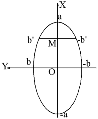
Schematic diagram of the contact width of the elliptic area at M.
Based on equation (22), we can get the removal depth of any point on the contact area and conclude that in different regions, the removal depths are different. Along the direction of the semi-major axis, the biggest removal depth happens on the center. The further away from the center, the smaller the removal depth becomes. The removal depth of the end point is 0. The schematic diagram of the removal depth along the direction of the semi-major axis is shown in Figure 3, which is almost the same shape with the results by Wang et al. 24 and Zhang et al. 25
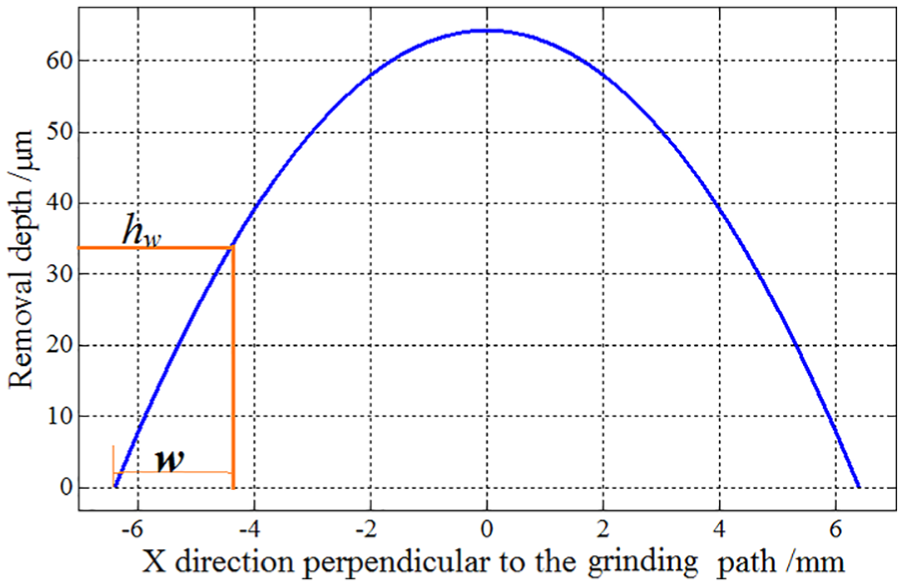
Schematic diagram of the removal depth.
In Figure 3, w represents the length away from the end point of the semi-major axis and hw is the removal depth at w.
The optimization model of tool-path planning
After grinding, there will be some unremoved material left between the two adjacent paths. The distance between the top of the material and the grinding surface is called the scallop-height. In precision machining, the scallop-height should be controlled within a certain range to guarantee the form accuracy of the workpiece. And, accordingly, under the situation that all the other parameters are held fixed (i.e. grinding force, modulus of elasticity, and Poisson’s ratio), two situations are contained in the tool-path planning:
If the maximum material removal depth of the workpiece is smaller than the threshold of scallop-height, then the full coverage model can meet the form accuracy and it is adopted in belt grinding. Under this circumstance, the grinding efficiency is the biggest;
If the maximum material removal depth of the workpiece is bigger than the threshold of scallop-height, then the full coverage model cannot meet the form accuracy. Under this circumstance, the tool-path interval needs to be optimized.
As for the second situation, it is assumed that the maximum material removal depth of the former path is hmax, which satisfies the following condition

where h is the threshold of scallop-height. And, the next path should overlap with the former one, which will remove the material between them and decrease hmax to meet the scallop-height.
The calculation of the tool-path interval based on the constant scallop-height method is as follows. Three situations are analyzed according to the curvature of the workpiece:
1. The tool-path interval of the plane surface.
The model is shown in Figure 4 and the detailed calculation method is as follows.

Schematic diagram of the scallop-height for plane surface.
It is assumed that the removal depth by the next path is h′ and then the scallop-height becomes

Then, the minimum removal depth by the next path is

Based on the model of the material removal depth, the removal depth of the removal outline 1 at any point can be obtained. We assume that at the point k, which is w away from the end point of the semi-major axis as shown in Figure 3, the removal depth hw is equal to hmax − h and the overlapped width is the value of w. Then, we can obtain the tool-path interval

2. The tool-path interval of the convex surface.
The model is shown in Figure 5 and the detailed calculation method is as follows.

Schematic diagram of the scallop-height for convex surface.
As shown in Figure 5, R is the principal radius of curvature of the workpiece at the local grinding place; O1 and O2 are the deepest points of outlines 1 and 2, respectively; L is the distance between O1 and O2, which is also the tool-path interval; G is the cross point of the removal outlines 1 and 2; the line O1N is the tangent line of the workpiece at the point O1, GN is perpendicular to O1N, and F is the cross point of line O1N and OG;
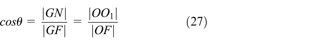
where

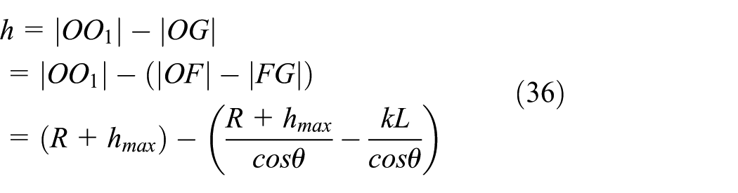
The scallop-height h can be expressed as follows

Substituting equation (28) into equation (29)

Since

where h is much smaller than R, so

Then, we can obtain the tool-path interval

3. The tool-path interval of the concave surface.
The model is shown in Figure 6 and the detailed calculation method is as follows.

Schematic diagram of the scallop-height for concave surface.
As shown in Figure 6, O1P is the maximum cutting depth

where
The shape of △OO1F is the function of L and the shape of outline 1 can be obtained by equation (22). The length of GN can be obtained through the cross point of △OO1F and outline 1 by the method of geometry, which will not be explained here due to the length limit of article.
As there is only one variable L which can affect the cross point, so

where k is a variable coefficient and can be obtained by the model of the material removal depth. Since
Then, we can obtain the expression of h as follows
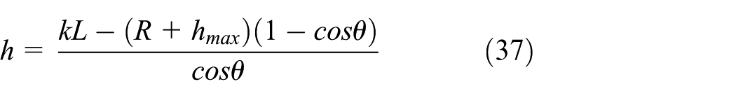
Under a certain threshold for h, the tool-path interval of the concave surface can be set as

Experiments and discussion
In the previous sections, a full coverage model and an optimization model for the grinding path were developed as shown in Figure 7. In this part, experiments are conducted to verify the models.
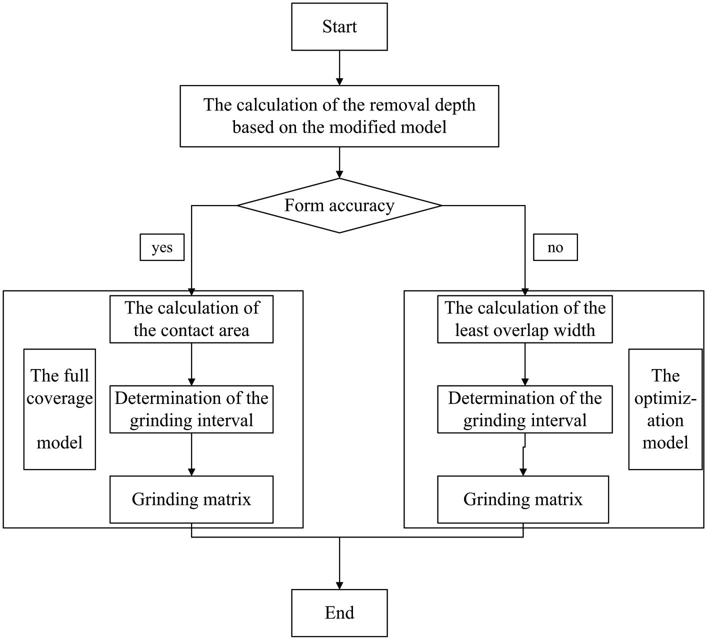
The schematic diagram of the grinding tool-path planning.
The free-form surface in this article is a simulation aero-engine blade as shown in Figure 8 and material of the workpiece is TC4. All the experiments were performed on the KUKA robot. Here, the force controller of ACF 110-10 produced by FerRobotics Company in Austria was used to control the grinding force. ACF is a flexible device that can automatically expand and contract according to the actual contact force to ensure a steady grinding force. In general, ACF is fixed at the end-effector of the robot as shown in Figure 9. Through the integration of multiple sensors, the reaction time of ACF can be as short as 4 ms, which guarantees that it can make feedback in real time to the robot and finally achieve precise control of the force through its control software.

The picture of the free-form blade in this experiment.

The usage of ACF on the robot.
The selection of grinding path mold
The aero-engine blade is chosen to the grinding object in the experiment. Generally speaking, there are two path molds in the blade grinding, namely, the transverse cutting method and longitudinal cutting method, as shown in Figure 10.

The schematic diagram of two path molds in the blade grinding: (a) transverse cutting method and (b) longitudinal cutting method.
The two kinds of grinding molds have their advantages in efficiency and quality, respectively. Here, in this article, the transverse cutting method is selected, as shown in Figure 11, in view of the following reasons. Residual knife marks can be brought to the surface of the blade after the grinding process to a certain degree, as shown in Figure 12. The blade is the flow channel for the high-pressure air, and the knife marks have a great influence on the flow properties of the air, which will further affect the service performance and life of the blade. Therefore, in order to improve the performance, the knife marks should have the same direction with the flow of the air.

Transverse cutting method in the blade grinding.

The profile of the residual knife marks.
The verification of the modified Preston model
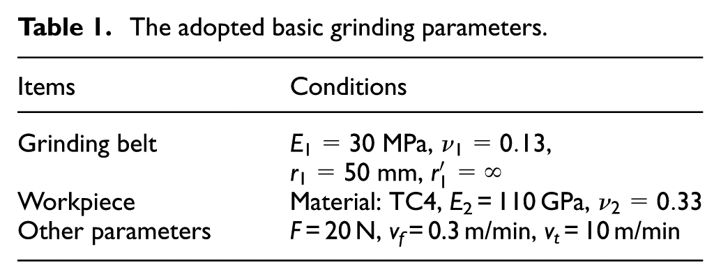
In order to verify the modified Preston model, a single-path grinding experiment on the blade is carried out. The basic parameters adopted in the experiments are listed in Table 1.
The adopted basic grinding parameters.
The profile admeasuring apparatus, InfiniteFocus G4 made by Alicona Company in Austria, is used to detect the removal result after the grinding. The surface profile after the grinding is shown in Figure 13(a). Perpendicular to the grinding path, the height of some points on the surface is recorded, and the difference before and after the grinding is the removal depth. Based on the MATLAB software, the removal profile is calculated and the curve fitting result is as shown in Figure 13(b), from which we can see that the experimental result is coincident with the theoretical result shown in Figure 3.

The experiment of the single-path grinding: (a) profile of the blade surface after grinding and (b) schematic diagram of removal depth.
The verification of the full coverage model
In this part, two groups of contrast experiments were carried out. One is the grinding path with the fixed interval and the other with the varied intervals. The schematic diagram of area coverage maps for the two conditions is shown in Figure 14. Obvious ungrinded areas in the red circles and over-grinded areas in the green circles can be seen from Figure 14(a), which is effectively improved in Figure 14(b). Known from the full coverage model, for the grinding of blade, the change of its curvature will lead to the change of the actual contact area. The fixed interval which considers only the geometry does not adapt to the change of curvature and can easily lead to the gap or overlap between the adjacent paths, which will result in increased manufacturing time and costs.

The schematic diagram of area coverage maps for different tool-path intervals: (a) fixed interval and (b) varied intervals.
Figure 15(a) shows the grinding surface under the fixed interval. In the yellow region, we can see that there are gaps between the adjacent paths and the smoothness is relatively poor, which verifies the results of Figure 14.

The experimental results under different grinding intervals: (a) fixed grinding interval, (b) full coverage model, and (c) optimization model.
The experiment result based on the full coverage model is shown in Figure 15(b). In this experiment, the grinding interval varied according to the change of the blade curvature. It can be seen that there are no obvious gaps on the surface. Therefore, the unground areas can be eliminated effectively by the model in this article, which proves that the model is with a good coverage.
The verification of the optimization model
The optimization model is based on the modified Preston equation. Therefore, the value of K should be calibrated by experiment first.
The calibration of the coefficient K
Known from the definition of Preston equation, once the characteristics of the grinding tool and workpiece material are fixed, K will be a constant and will not change. Therefore, its value has nothing to do with the grinding mold, and the dwell grinding mold is adopted here.
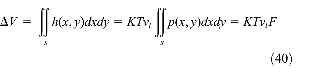
Based on the Preston equation, the removal volume during time T can be expressed as

Combined with the Hertzian contact theory, equation (39) can be calculated as follows
Therefore, the expression of K can be obtained in the following form
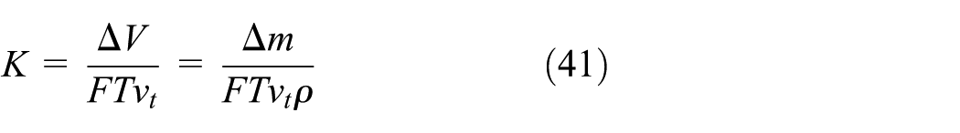
where
Based on the analyses above, the dwell experiments of TC4 surface plate were carried out as shown in Figure 16. As stated above, K is a constant under the fixed grinding condition. Then, in order to reduce the random error, six groups of experiments were carried out. In the experiments, the processing parameters, namely, normal contact force F, dwell time T, and belt speed vt, varied and the change of mass was measured by a precision electronic balance. The processing parameters and experimental results of the plate dwell experiments are shown in Table 2.

The experiment of the dwell grinding on a TC4 surface plate: (a) schematic diagram of the dwell experiment and (b) experiment of dwell grinding.
The processing parameters and experimental results of the plate dwell experiments.

According to equation (41), the value of K can be determined by the linear fitting of the experimental results, and the final result of K turns out to be 2.11 × 10⁻¹¹.
The verification of the optimization model
In order to show the effectiveness of the optimization model, two groups of contrast experiments were also carried out here. Figure 15(c) shows the grinding surface based on the optimization model. Compared with Figure 15(b), we can find that there are no obvious gaps in the two grinding situations, from which we can conclude that the two models in this article can both efficiently avoid the grinding gap. We analyzed the advantage of the optimization model by the comparison of the areas in the yellow line in detail. In the yellow area of Figure 15(b), there are slight bulges. They are eliminated in Figure 15(c) and the grinding surface is smoother. In order to show the comparison clearly, the InfiniteFocus G4 is used to detect the micro-morphology of the two grinding surfaces, and the results are shown in Figure 17.

The micro-morphologies based on different tool-path planning models: (a) full coverage model and (b) optimization model.
It can be clearly seen from Figure 17(a) that the morphology in the yellow area has obvious difference with that of the two sides. It can be explained that when adopting the full coverage model, the removal depth at the very edge of the path is zero. Then, when the total removal depth is relatively big, it is easy to lead to an obvious scallop-height and the profile in the yellow area is shown in Figure 18(a). Compared with Figure 17(a), the micro-morphology in Figure 17(b) is smoother and no obvious scallop-height can be seen as shown in Figure 18(b). Therefore, we can conclude that the optimization model can effectively reduce the scallop-height and improve the form accuracy of the workpiece.

The micro-profiles of different path planning models: (a) full coverage model and (b) optimization model.
Conclusion
In this article, based on the contact theory and taking the grinding force into consideration, tool-path planning is studied as a contact mechanical problem in belt grinding. A model of full coverage is developed, and moreover, an optimization model for the interval is presented. Summarized in the following are the major contributions:
Taking the grinding force and the characteristics of the grinding belt and workpiece into consideration, a real contact area model for the interaction between the grinding belt and the workpiece surface is developed based on the Hertzian contact theory.
Based on the area model, a full coverage model of the tool-path planning for free-form surface is developed and the matrix of the coordinates along the X-axis direction of all the contact points is presented.
Based on the Preston equation, the calculation equation for the linear removal intensity is derived and the model of the material removal depth is established finally.
Taking the requirement of the scallop-height into account, an optimization model for the interval is presented to meet the high-accuracy requirement of the workpiece. According to the curvature of the contact surface, three situations are analyzed and the calculation methods of the tool-path interval are given.
Experiments are conducted on the simulation blade. The results show the effectiveness of the tool-path planning methods developed in this article.
The models in this article can be used as the theoretical foundation for the selection of the interval in tool-path planning to achieve high efficiency and form accuracy. The models proposed in this article may be helpful for the improvement and development of the automatic grinding system.
Footnotes
Handling Editor: Xichun Luo
Declaration of conflicting interests
The author(s) declared no potential conflicts of interest with respect to the research, authorship, and/or publication of this article.
Funding
The author(s) disclosed receipt of the following financial support for the research, authorship, and/or publication of this article: This study was supported by the Science & Technology Coordination & Innovation Project of Shaanxi Province (No. 2016TZC-G-15-2).