Sage Journals: Discover world-class research

Abstract

Pipeline is important for gas transportation. Free span of buried pipeline may cause safety problem as a result of decreasing the load-carrying capacity of the pipeline. A method for detecting the free span of buried pipelines based on the inner pipe excitation signal was proposed. Vibration characteristics analysis of the pipe and its surrounding coupling system were discussed by means of the finite element method. A three-dimensional pipe model containing a free-spanning segment with a certain length was established. Transient dynamic response analysis was adopted. Frequency response function plots were generated to analyze the results of simulation. The effects of soil type, the length of the free-spanning segment, and the excitation signal on detection were studied. The results show that (1) the obvious change of the first natural frequency of the pipe with different surroundings can be used to detect the free-spanning segment of pipeline; (2) the harder the soil medium is, the higher the first natural frequency of the pipe and soil surrounding system will be; (3) the longer the length of the free-spanning segment is, the lower the first natural frequency will be.

Keywords

ANSYS excitation signal transient dynamic response analysis free-spanning pipe pipe–soil coupling

Introduction

Gas pipeline is always placed under the ground. Free spans of buried gas pipelines may develop gradually due to landslide, soil settlement, and so on. As the length of the free-spanning segments increases and the resistance of pipeline to deformation weakens, the free span of pipelines is more vulnerable to load change such as pressure and crust movement. Therefore, the detection of free spans of buried pipeline is important.^1–3

The existing technologies for detecting the support conditions of buried pipelines mainly include ray detection, ultrasonic detection, and so on. At present, the total distance of China’s oil and gas pipelines has reached 120,000 km. These methods are constantly affected by complex external environment, and reliability of testing cannot be guaranteed since they are outer pipeline detecting methods. So, an inner pipeline method for detecting support conditions of buried pipelines becomes a trend. With the development of detecting technology, the British Natural Gas Online Testing Center has developed a nuclear energy pipeline testing device. By analyzing the characteristics of the interaction between the neutron beam and the surrounding medium emitted by the neutron source on the pig, the support conditions of the pipeline can be determined. However, the difficulty of remote data transmission during the long-distance pipeline detection limits its application.^4,5 An inner pipeline method for detecting the support conditions of buried pipelines based on forced vibration signal analysis is proposed in this study. The detection device consists of three parts: vibration generator, signal acquisition, and battery. Vibration generator can generate excitation signal. Vibration response signal collected by acceleration sensors is stored in the signal acquisition warehouse. This detection device is dragged by Pipeline Inspecting Gauge (PIG), as shown in Figure 1. The smart PIG has the function of speed control by drainage. Operation parameters of smart PIG, such as frequency of speed governing and threshold, were preset according to the pressure and flow rate of natural gas in the pipeline and the diameter and route of pipeline. Smart PIG can stop after moving a distance and hold on. At the same time, the excitation force of detection device will be applied on pipeline for just 2–3 s. And then, the smart PIG will be restarted. This method not only reduces the interference of the external environment on the testing process but also can simultaneously analyze the excitation signal and the response signal.^6–8

Figure 1.

Detection device of pipeline.

Based on ANSYS Workbench finite element analysis software, a three-dimensional pipeline model with free-spanning segment was established in this study. Sine sweep signal was selected as excitation signal. The transient dynamic response of pipeline under different support conditions was studied. It can be concluded that this method can detect the support conditions of the pipelines and distinguish the free-spanning segment of buried pipeline by analyzing the frequency response function (FRF). At the same time, to further explore detection effect under different conditions, soil type, length of free-spanning segment, and excitation signal were selected as variables in this study.

Finite element model

Model establishment and parameter setting

In this article, gas pipeline with free-spanning segment in service was used as simulation research object. Interaction between pipeline and soil is concerned in the processing of establishment of the model. Defects and weld on the surface of the pipeline were neglected in this study. The model was a pipe with an outer diameter of 0.355 m and a wall thickness of 0.005 m. The parameters of pipeline, effective density (ρ), elastic modulus (E), and Poisson’s ratio (μ), used were ρ = 7850 kg/m³, E = 2 × 10¹¹ Pa, and μ = 0.3, respectively. Since the wall thickness was much smaller than the radius of curvature in the middle of the pipe, the pipe can be treated as a thin shell. So, conceptual modeling method in ANSYS Workbench was adopted to establish the model.

Contact setting

In the simulation, the nonlinear spring (soil spring) with damper was used to simulate the coupling between the pipe and soil.^9–13 By setting the spring stiffness and damping coefficient, the soil supporting the pipeline can be simulated. In order to facilitate the analysis and calculation, following assumptions were made in this study:

The soil adjacent to the free-spanning segment did not slip or collapse, which can be regarded as a fixed state;

The pipe is laid horizontally. There was no height difference in the vertical direction.

The length of the buried segment in reality is so long that could not be shown completely in the simulation. In order to find out the optimal length of the supported segment, several simulations with supporting length of 1, 3, 5, 7, 9, 11, 13, 15, and 17 m under free-spanning length of 1, 3, 5, 7, 9, 11, 13, and 15 m had been done. According to the simulations, it can be known that for the pipe used in this model, the FRF of the buried segment no longer changes obviously when the length of the buried segment is more than 7 m under a certain free-spanning length. So, it could be recognized that the supporting effect due to the buried segment of 7 m length was equivalent to the supporting effect of the infinite buried segment. Therefore, the pipe–soil coupling length was set to be 7 m, that is, there were soil springs along the pipe axis with the length of 7 m at both ends of pipe. The length of free-spanning segment was 7 m in this simulation. Further study of effect of free-spanning length on detection is described in detail below.

Considering the excitation force applied on the lowest point of the pipe along the vertical direction, the pipe will be mainly affected in the vertical direction of the surrounding soil. The outer wall of the pipeline distributed two horizontal and vertical soil springs along the radial direction, which represent the stiffness of the soil,^14–17 as shown in Figure 2. One end of the spring unit was connected to the pipe and the other end was fixed. In the simulation, the stiffness and damping coefficient of middle-sized sand were used as the simulation parameters. The damping coefficient (c) and the spring rate coefficient (K) were c = 0.3 and K = 1.0×10⁶ N/m in accordance with Bloem.¹⁸

Figure 2.

Spring and damping distribution.

Boundary condition

Two kinds of boundary conditions at both ends of the pipe were proposed:

Four soil springs along the axis of the pipe were uniformly distributed on both ends of the pipe. The longitudinal stiffness (K_l) and torsional stiffness (K_t) of springs were K_l = 3.0 × 10⁸ N/m and K_t = 3.0 × 10⁸ N m/rad. The damping coefficient was set to 3.0.⁹ One end of the spring was connected to the pipe and the other end is fixed.

One end of pipe had no springs along the axis and fixed support was adopted on it. The other end was connected with four uniformly distributed soil springs along the axis of the pipe. The parameters of spring used were K_l = 3.0 × 10⁸ N/m and K_t = 3.0 × 10⁸ N m/rad. The damping coefficient was set to 3.0.

The simulations with two different boundary conditions under the supporting lengths of 3, 5, 7, 9 m and free-spanning length of 7 m were studied, respectively. According to the simulation, it can be known that the vibration response of the pipeline under excitation signal is basically the same under the two boundary conditions. However, it had high calculation efficiency when the first boundary condition was selected. So, the first boundary condition was adopted in the following simulation.

Meshing

Shell 181 was adopted in the pipe model. The grid is hexahedral, which is suitable for analyzing moderately thick shell structures. The grid size was set to 0.2 m, and the finite element model is shown in Figure 3. In this model, the spring and damping device are integrative. That is to say, the spring stiffness and the damping coefficient were set at the same time to obtain the spring damping unit, which is different from the distribution in Figure 2.

Figure 3.

Pipeline finite element model.

Dynamics simulation

Parameter setting of dynamic analysis

Transient dynamic analysis method was used to study the vibration response characteristics of two different support conditions of pipeline based on forced vibration signal in the pipe. This method is used to determine the structural dynamic response under any load varying over time. Considering the sin sweep signal and the nonlinear characteristics of the soil spring structure, transient dynamic analysis method was adopted in this study.

This study was conducted to verify the applicability of this method and identify the free span of buried pipeline. The static detecting method was adopted in the simulation. Because the measuring procedure can be realized, the movement of the PIG not considered too. Excitation signal was only applied on one point in one simulation, and the acceleration response of this point was obtained. The detection point and the excitation point are the same. In total, 20 detecting points in the pipeline were selected. The first detecting position was located at 1 m. And then, the remaining detecting points are taken along the pipeline with the spacing of 1 m until 20 m. They were named 1 to 20 in sequence, as shown in Figure 4.

Figure 4.

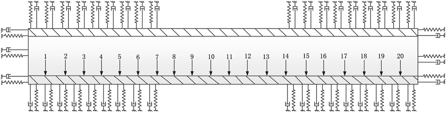
Distribution of detection points.

In this article, the sine sweep signal was used as the excitation signal. The sample frequency was set to 1652 Hz. The steady-state sinusoidal sweep was the optimal method for the system excitation and the acquisition of transfer function. The excitation power generated by this method is large. The signal–noise ratio in the process of calculation result is high. So, this method can obtain higher testing accuracy, which has greater advantages compared with other exciting method. This method is not only generally used to detect the reliability of product structure but also used for structural damage detection.^11,19 In the simulation, the sweep range was taken as 1–300 Hz. The sweep rate was set to 1 Hz and the value of excitation force was 0.3 N in this simulation, as shown in Figure 5. The excitation force amplitude parameter was studied in the following simulations. The acceleration response of the point which excitation force was applied on is the desired vibration response of the system. Taking detecting point 3 as an example, Figure 6 shows that the time-domain and frequency-domain maps of the acceleration response at point 3 when the excitation force acts on point 3.

Figure 5.

Sine sweep signal: (a) time domain and (b) frequency domain.

Figure 6.

Acceleration response: (a) time domain and (b) frequency domain.

Analysis of vibration response

The FRF spectrum of the vibration response signal is obtained by MATLAB. Figure 7(a)–(c) is the FRFs of the detection points 2, 10, and 6, respectively, on the pipeline. The detection points 11, 20 and the detection points 1, 10 were symmetrical points. Their FRF spectra are basically the same. The first natural frequency of the free span is about 20 Hz, that is, the frequency at which the peak ① in Figure 7 was located. The first natural frequency of the buried segments was about 75 Hz, that is, the frequency at which the peak ③ in Figure 7 was located. It can be known from Figure 7(a) and (b) that the peak ③ has a significant right shift compared with the peak ①. The first natural frequency had a significant change. This shows that the method introduced in this article can distinguish between the well-supported and free-spanning segments. If two different conditions of the pipeline were regarded as a complete system, it can be assumed that the peak ① was the dominant frequency of the free span and the peak ③ was the dominant frequency of the well-supported segments. Figure 7(c) shows the FRF of the detection point 6, which is located near the junction between the well-supported and the free-spanning segments. The peak ② between the peaks ① and ③ appears in the spectrum at a frequency of about 49 Hz. At the same time, it can be seen that the diagram contains the dominant frequency of the well-supported and the free-spanning segments, indicating that the detecting point has both the characteristics of the two different conditions of pipeline. But the amplitude of peaks ① and ③ compared with the peak ② was much smaller. The frequency at the peak can be considered as the dominant frequency of this part. In this article, the part of pipe with this kind of characteristic was defined as the transition section of well-supported and free-spanning segments.

Figure 7.

FRF of different conditions of pipeline: (a) free span (point 10), (b) well-supported segment (point 2), and (c) transition segment (point 6).

Figure 8 shows the first natural frequency distribution of each detection point. It can be seen that the figure is in a staircase shape. This result was similar to the “ladder shape” shown in the gray plots of FRFs obtained by NS Liao’s experiments. Although the steel plate was used as a substitute of pipe, the detecting method based on excitation signal was verified and the free span of pipeline can be identified. The first natural frequency of each detection point in the same section basically remains unchanged, and the first natural frequencies of the detection points in different sections had obvious differences. The first natural frequency of the free span changes obviously compared with the well-supported segments. The specific value of the first natural frequency is no need to be obtained, since pipeline has different vibration characteristics under different supporting conditions. But a significant difference of first natural frequency between well-supported and free-spanning segments is what should be focused on. Therefore, the condition of the pipeline at the detection point can be determined according to the first natural frequency of the detected point, to judge whether the pipeline was in a free-spanning condition.

Figure 8.

First natural frequency distribution of each detection point.

Results and analysis

Influence of soil spring stiffness on detection

The environment in which the pipeline is located is very complicated. Due to the different geological soils, the character of the supporting medium outside the pipe was also greatly different. Further exploration of the effect of different supporting media on the free span detection simulations under different types of soil has been done by changing the spring stiffness parameters in the model. The detection effect of this method under different support conditions is obtained.²⁰ Vertical excitation signal was applied in this method, so the circumferential springs of the pipeline have a great influence on the dynamic response of the pipeline. Therefore, it was to maintain the same boundary conditions and only to change the stiffness of the soil springs. At the same time, the length of the free-spanning and buried segments was all 7 m. In the simulation, the sweep range was taken as 1–300 Hz. The sweep rate was set to 1 Hz and the value of exciting force was 0.3 N. The damping coefficient of the soil spring was 0.3.

The coefficient of soil stiffness can be obtained from the elastic modulus of the soil. The calculated stiffness (K_s) of the soil was K_s = 5.89 × 10⁵ N/m.²¹ Six different types of supporting media were selected. The stiffness coefficient of each is shown in Table 1.^12,22 Under different soil spring stiffness values, the corresponding first natural frequency of the well-supported and the free-spanning segments is shown in Figure 9.

Table 1.

Calculated stiffness of different supporting media.

Type of soil	Soft clay	Hard clay	Breaking up sand	Pack sand	Hard sand	Stone
$K_{s} (N / m)$	1.0 × 10⁵	5.0 × 10⁵	1.0 × 10⁶	2.0 × 10⁶	3.0 × 10⁶	4.0 × 10⁶

Figure 9.

First natural frequency of free-spanning and well-supported segments under different supporting media.

It can be seen from Figure 9 that when $K < 1.0 \times 10^{6} N / m$ , the stiffness had more effect on the first natural frequency of the well-supported segment than free-spanning segment. When $K \geq 1.0 \times 10^{6} N / m$ , there was almost no change in the first natural frequency of the free-spanning and well-supported segments. When $K < 1.0 \times 10^{6} N / m$ , the first natural frequency of two different supporting conditions of the pipeline does not change much. The detection method based on the excitation signal in the pipeline was more effective when the supporting media was sand. The difference of first natural frequency between free-spanning and well-supported segments was less when the supporting media was soft such as clay. The harder the soil, the higher the first natural frequency of the well-supported segment and the more obvious difference with the free-spanning segment. It can get the better recognition of the free-spanning condition.

Influence of the length of the free span on detection

In order to find out the detection effect of free-spanning lengths of pipeline on detection, the spring stiffness along the axial direction at both ends of the pipe is K = 3.0×10¹¹ N/m, and the spring stiffness of the circumferentially distributed soil springs at both ends of the pipe is K = 1.0 × 10⁶ N/m. The damping coefficient of soil spring is 0.3. And, the length of supporting section at both ends of pipe is kept at 7 m. So, the effect of the detection under different lengths of free span was obtained.^23–26 Lengths of the free span were chose as 0.5, 1, 2, 3, 4, 5, 6, 7, 8, 9, 10, 11, and 12 m. The first natural frequency of two different supporting conditions of pipeline is shown as Figure 10.

Figure 10.

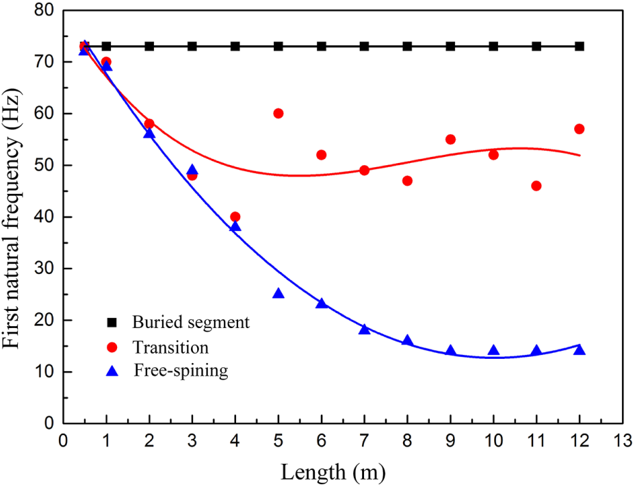
First natural frequency of free-spanning and well-supported segments under different lengths of free span.

It can be seen from Figure 10 that the first natural frequency of the free span decreases with the increase in the free-spanning length of the pipeline when the length. The first natural frequencies of the transitional section and free span were almost the same when the suspended length was less than 4 m. The vibrational characteristics of the transitional section were similar to those of the free span. When the length of free span was more than 4 m, the first natural frequency of the transition section fluctuates with the increase in the length of free span. Comparing the first natural frequency of the free span section with the well-supported section, when the length of free span was less than 2 m, there was less difference between the different supporting segments. The detection method cannot effectively identify the free span of the pipeline. When the length of free span was more than 2 m, this method can distinguish two different supporting conditions well and detect the free span of the pipeline.

Influence of excitation signal on detection

In order to detect more effectively, the influence of excitation signal parameters on the detection effect was also studied in this article. Excitation force amplitude and sweep rate were two important parameters of excitation in detection. Amplitude of the excitation force should be high enough to excite the pipe and stable response signal could be obtained. Sweep rate means the sweep times of the frequency range in a unit time. The sweep rate should be selected to ensure both the stability of accelerate response and the minimum time cost. The free span length was 7 m and the spring constant was K = 1.0×10⁶ N/m. Table 2 shows the change of excitation force parameters. Table 3 shows the change of sine sweep rate.

Table 2.

The change of excitation force.

Excitation force (N)	Sweep rate (Hz)	Sweep range (Hz)
0.1	1	1 ~ 300
0.2	1	1 ~ 300
0.3	1	1 ~ 300
0.4	1	1 ~ 300
0.5	1	1 ~ 300

Table 3.

The change of signal sweep rate.

Excitation force (N)	Sweep rate (Hz)	Sweep range (Hz)
0.3	0.5	1 ~ 300
0.3	1	1 ~ 300
0.3	2	1 ~ 300
0.3	4	1 ~ 300
0.3	8	1 ~ 300

When the excitation force increased from 0.1 to 0.5 N, the FRF of free-spanning and well-supported segments was almost the same. The excitation force had less influence on the detection when it can excite the system. However, the pipeline was in an ideal condition in the simulation. The effect of the fluids and deposits in the pipeline on the excitation signal, and the attenuation and absorption of the excitation signal on the pipe wall and soil were all neglected. Under real working condition, in order to reduce the influence of the above factors on detection, it was better to use a larger excitation force without any damage to the pipeline.

When the sweep rate increases from 0.5 to 8 Hz, the first natural frequency of the free-spanning and the well-supported segments obtained at each sweep rate obviously changed. It is indicating that the change of the sweep rate in this range had no impact on the suspended state of the pipeline. At the same time, the first natural frequencies of the free-spanning and the well-supported segments obtained by different sweep rates had basically not changed. However, it can be seen from Figure 11 that when the sweep rate was too small or too large, the FRF was obviously fluctuated and disturbed. When the sweep rate was less than 0.5 Hz and the sweep rate is increased, the curve obviously has interference and becomes non-smooth. It was difficult to compare and analyze the response characteristic of the pipe. Therefore, in order to more clearly observe the natural frequency peak, the sweep rate should be chosen about 1 Hz.

Figure 11.

FRF of point 10 under different sweep frequencies: (a) 0.5 Hz, (b) 8 Hz, and (c) 1 Hz.

Conclusion

In this article, the three-dimensional finite element model of pipeline with free-spanning and buried segments was established by ANSYS Workbench. And, transient dynamics analysis on pipeline was obtained. Meanwhile, the method of free span of pipeline detection based on excitation signal was analyzed under different free-spanning lengths, different types of soil, and different excitation signals. The following conclusions can be given:

Through the comparison between the vibration characteristics of the free-spanning and the well-supported segments, the first natural frequency in the FRF of the free-spanning and the well-supported segments has a significant difference. It can be considered that this detection method can effectively identify the free-spanning condition of pipeline;

The harder the soil in the buried segments of pipeline, the larger the first natural frequency of the well-supported segments and the better the detection effect on the free-spanning condition. The softer the soil, though the difference between the first natural frequencies of two different supporting conditions is not obvious, the detection of the free span of the pipeline can also be achieved;

The longer the length of free span is, the smaller the first-order natural frequency of this segment is. The more obvious the difference between the vibration response characteristics of the free-spanning and the well-supported segments is, the better the identifying effect of the detecting method is. When the length of free span is greater than 9 m, the first natural frequency no longer changes obviously with the length. When the free span length is less than 2 m, the free span is greatly affected by the vibration characteristics of the buried segments. The detection method cannot identify the short-distance suspended section;

The value of the excitation force has no effect on the detection when it can excite the system. When the excitation signal sweep rate is too large or too small, the FRF spectrum has significant fluctuations in the results of the analysis and processing. The sweep frequency of 1 Hz is most appropriate.

Footnotes

Handling Editor: Dumitru Baleanu

Declaration of conflicting interests

The author(s) declared no potential conflicts of interest with respect to the research, authorship, and/or publication of this article.

Funding

The author(s) disclosed receipt of the following financial support for the research, authorship, and/or publication of this article: This work was financially supported by the National Natural Science Foundation of China (No. 51805542) and the Science Foundation of China University of Petroleum, Beijing (No. 2462017YJRC001).

ORCID iD

Hang Zhang

References

Leckie

SHF

Draper

White

et al . Lifelong embedment and spanning of a pipeline on a mobile seabed. Coast Eng 2015; 95: 130–146.

Liu

Wang

et al . Composite magnetic flux leakage detection method for pipelines using alternating magnetic field excitation. NDT&E Int 2017; 91: 148–155.

Shahverdi

Lotfollahiyaghin

Shahverdi

Subsea free span pipeline damage detection based on wavelet transform under environmental load. J Persian Gulf 2013; 4: 51–64.

Xue

Hong

A numerical study of damage detection of underwater pipeline using vibration-based method. Int J Struct Stab Dy 2012; 12: 1250021.

Liu

JF.

Analysis of vibration problems during the detection of submarine pipelines. Saf Healthy Environ 2018; 18: 37–40.

Liao

Ding

Jr Zhang

et al . A method for identifying free span of subsea pipelines. In: The 27th international ocean and polar engineering conference, San Francisco, CA, 25–30 June 2017. US: International Society of Offshore and Polar Engineers.

Neto

Cavalini

Jr Vedovoto

et al . Influence of seabed proximity on the vibration responses of a pipeline accounting for fluid-structure interaction. Mech Syst Signal Pr 2019; 114: 224–238.

Zhao

Guan

Dong

et al . Correction and inspection of submarine pipeline span in the Chengdao oil field. Coast Eng 2012; 31: 14–20.

Gao

Xie

Prediction model of multi-span pipelines subjected to vortex induced vibration (VIV) in cross flow. Mar Eng 2016; 34: 41–46.

10.

Gao

Wang

et al . Pipe-soil interaction model for current-induced pipeline instability on a sloping sandy seabed. Can Geotech J 2016; 53: 1822–1830.

11.

Ansari

Kouretzis

Sloan

SW.

Development of a prototype for modelling soil–pipe interaction and its application for predicting uplift resistance to buried pipe movements in sand. Can Geotech J 2018; 55: 1451–1474.

12.

Peche

Graf

Fuchs

et al . A coupled approach for the three-dimensional simulation of pipe leakage in variably saturated soil. J Hydrol 2017; 555: 569–585.

13.

Naggar

MHE

Abdlrahem

et al . New interaction model for vertical dynamic response of pipe piles considering soil plug effect. Can Geotech J 2017; 54: 987–1001.

14.

Wijewickreme

Monroy

Honegger

et al . Soil restraints on buried pipelines subjected to reverse-fault displacement. Can Geotech J 2017; 54: 1472–1481.

15.

Giannini

Casini

Vestroni

Nonlinear harmonic identification of breathing cracks in beams. Comput Struct 2013; 129: 166–177.

16.

Sarvanis

Karamanos

Vazouras

et al . Permanent earthquake-induced actions in buried pipelines: numerical modeling and experimental verification. Earthq Eng Struct D 2018; 47: 1032–1053.

17.

Zakeri

Submarine debris flow impact on suspended (free-span) pipelines: normal and longitudinal drag forces. Ocean Eng 2009; 36: 489–499.

18.

Bloem

Drag forces caused by submarine glide block or out-runner block impact on suspended (free-span) pipelines: numerical analysis. Ocean Eng 2013; 67: 89–99.

19.

Niu

Yan

X. A

FFT-based variety-sampling-rate sine-sweep vibration controller. In: Proceedings of the international conference on neural networks and signal processing, Nanjing, China, 14–17 December 2003, vol. 2, pp.1714–1718. New York: IEEE.

20.

Slingsby

Dynamic interaction of subsea pipeline spans due to vortex-induced vibrations. Master’s Thesis, Delft University of Technology, Delft, 2015.

21.

Vedeld

Sollund

Hellesland

Free vibrations of free spanning offshore pipelines. Eng Struct 2013; 56: 68–82.

22.

Sollund

Vedeld

Fyrileiv

Modal response of short pipeline spans on partial elastic foundations. Ocean Eng 2015; 105: 217–230.

23.

Ajdehak

Zhao

Cheng

et al . Numerical investigation of local scour beneath a sagging subsea pipeline in steady currents. Coast Eng 2018; 136: 106–118.

24.

Wang

Zhao

et al . Allowable span length of submarine pipeline in shallow water. Mar Georesour Geotec 2017; 36: 532–539.

25.

Furnes

Berntsen

On the response of a free span pipeline subjected to ocean currents. Ocean Eng 2003; 30: 1553–1577.

26.

Yang

Guo

Lou

et al . Allowable span length of submarine pipeline considering damping. Ocean Eng 2005; 23: 1–5.

Vibration response analysis of free-spanning pipeline based on inner pipe excitation signal

Abstract

Keywords

Introduction

Finite element model

Model establishment and parameter setting

Contact setting

Boundary condition

Meshing

Dynamics simulation

Parameter setting of dynamic analysis

Analysis of vibration response

Results and analysis

Influence of soil spring stiffness on detection

Influence of the length of the free span on detection

Influence of excitation signal on detection

Conclusion

Footnotes

Declaration of conflicting interests

Funding

ORCID iD

References