Sage Journals: Discover world-class research

Abstract

Time-domain or transient dynamic response method is the most traditional method used to evaluate the dynamic response of a vibratory system subjected to deterministic inputs. The inertia or damping effects are very crucial in the time scale of loading. The present work determines the time domain analysis of railway locomotive using finite element analysis for Indian tracks. The track inputs are modelled as an ellipsoidal bump, and variations in displacement at different key locations of the truck and carbody models are plotted subjected to standard loading conditions. The response plot of the front and rear locations of the locomotive truck and carbody indicate that these regions are more responsive to wheel inputs in comparison to the mid portion due to unbalanced mass distribution. In the further study vertical-lateral random inputs are measured through track recording car and modelled to express in the form of PSD. These random inputs are provided to finite element modelled flexible bogie frame, and acceleration response is determined. The results obtained are compared with the same obtained from rigid bogie frame formulated using an analytical model. The results obtained from the flexible and rigid body models are found to be in good agreement.

Keywords

Dynamic analysis vibrations transient response FE model ANSYS

Introduction

The time domain method may be used for both linear and nonlinear vibratory systems. This method can efficiently analyze the time-dependent response, strains, stresses, and forces for a system as it responds to combined static, dynamic, transient, or steady-state loads. The time domain method uses the general governing equation of motion as below.

[M] {\ddot{u}} + [C] \dot{{u}} + [K] {u} = F (t)

(1)

Time-domain transient vibrations^1–3 usually occur when a system is excited by a sudden, non-periodic excitation. The magnitude of such oscillations varies based on the type of excitation, and they occur at the system’s natural frequencies. Time-domain transient vibrations could be observed in railway vehicle vibrations, when the system is subjected to a few specific inputs that is bump, cusp, trough, and pothole inputs.

From the results obtained through FE analysis^4–6 it was concluded that the time domain method may be effectively used to analyze the rail vehicle behavior subjected to real-time input excitations as the vehicle traverses a semicircular bump. Lateral and vertical responses of the bogie or truck model^7,8 were plotted against time. The lateral displacement of the first axle of the five DOF bogie model⁷ was plotted against time at a speed of 66.22 m/s, considering a defect amplitude varying from 1.9 mm to 2.1 mm wavelength of 18 m.

Researchers^9–13 obtained time history response in terms of displacement, acceleration, velocity and contact forces at the wheel-rail interaction for rail vehicles under the influence of wheel flats. For the 10 DOF vehicle-track coupled model¹⁴ axle acceleration and the variations in wheel-rail contact force^7,15 were plotted against time, whereas the transient response was obtained for the five DOF vehicle-track model¹⁶ in terms of displacement, velocity, acceleration and wheel-rail contact forces considered a single irregularity either due to bad welded joint or settlement of ballast. The time history of numerical velocities for the FE model of EMU train¹⁷ in the vertical direction is plotted considering (a) without defect and (b) with a ramp irregularity. Harak et al.¹⁸ carried out finite element analysis of open type freight wagon “BOXN25” of the Indian Railways. The freight wagon vehicle was considered to consist of car body and two bogie frames. Solidworks was employed for modeling and the geometry was exported to finite element tool, ANSYS. Lu et al.¹⁹ investigated the influences of vibration modes on fatigue damage in bogie frames of high-speed railway vehicles. Lee et al.²⁰ presented an approach to upgrade a bogie suspension (without damaging) and to improve the vibration isolation of a carbody in the infra frequency range, which is crucial to improve ride comfort.

Bogie Pivot transmits the tractive/braking forces and also bears the vertical load of carbody. So, the sensor is installed at the railway vehicle’s bogie pivot during experimental acceleration measurements, and that location indicates the acceleration of the carbody. Every calculation made using the analytical method refers to the mass centre of rigid bodies. The major benefit of this approach is that Finite Element analysis makes it simple to evaluate the kinematic parameters, such as displacement and accelerations at various locations for the vehicle body, with reasonable precision.^21,22

In the present work, geometric CAD model of railway truck/bogie frame of Indian railway ICF (Integrated Coach Factory) passenger sleeper coach is developed and further translated to finite element ANSYS model. The time domain transient behavior of the system under bump inputs is analyzed at different locations of the system. In the further study, a rigid body model of the railway vehicle is formulated using an analytical method. The results obtained from rigid model analysis are compared with the equivalent finite element flexible model of truck/bogie frame subjected to random track inputs. The results obtained were found to be in good agreement; therefore the modelling is validated.

Modelling and simulation

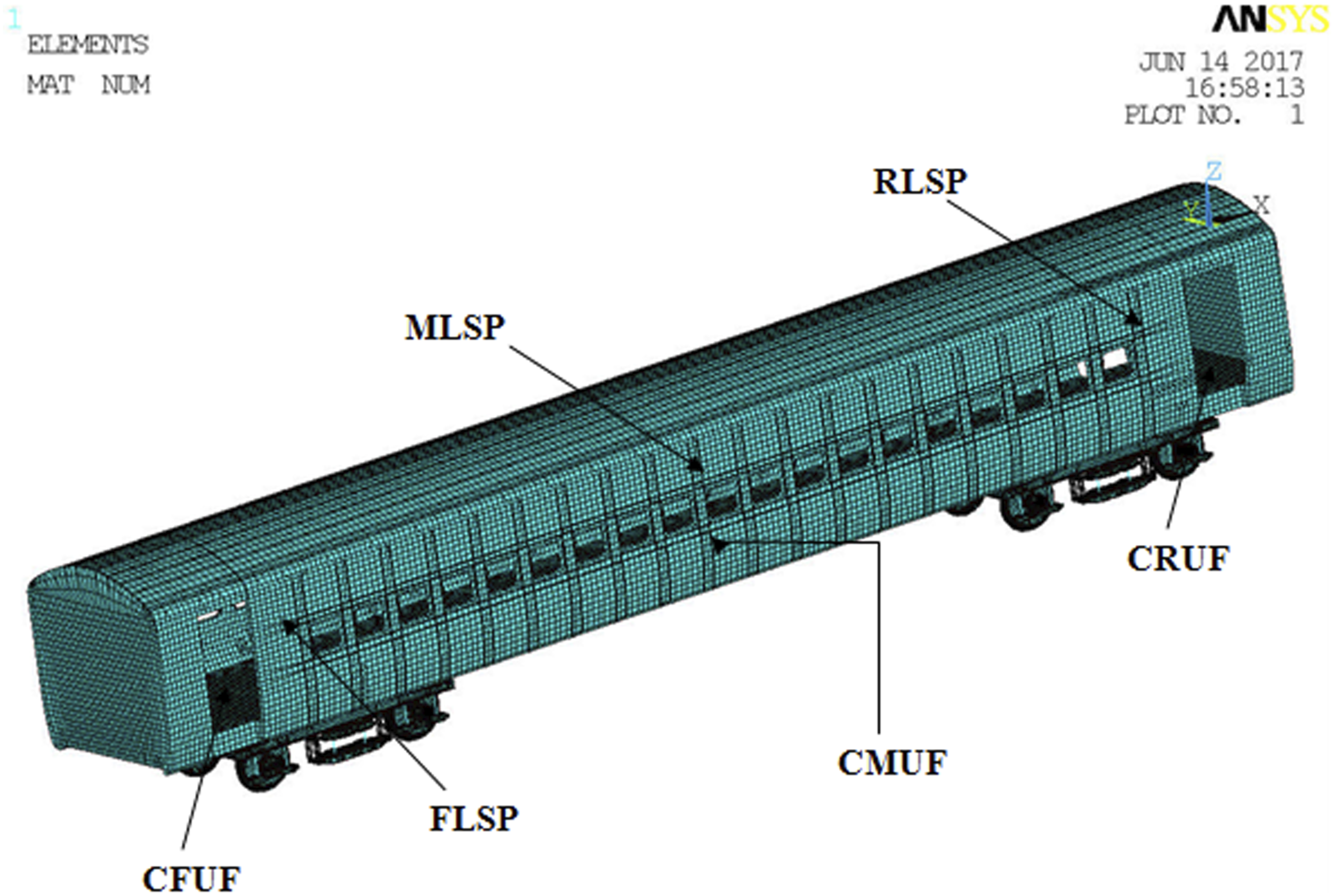
The present work considers an Indian railway ICF (Integrated Coach Factory) passenger sleeper coach. Geometric models of the Bogie or Truck as well as the coach are developed in NX 7.5 CAD software. These geometric models are further translated as finite element models to carry out the required analysis in FEA software ANSYS APDL 12.1. The truck frame, bolster, and wheel axle sets are modelled as solid elements using SOLID92 (Figure 1). The suspension elements are modelled as spring elements with COMBIN14 element. The truck model is discretized with Automatic mesh generation with tetrahedral elements. The coach shell with the channels such as sole bars, stanchions etc are meshed using SHELL 63. The discretized railway coach model along with the defined suspensions and element types is shown in Figure 2. A bump with a maximum height of 10 mm is modelled considering the standard assumptions that the time consumed for the bogie to traverse the bump is 0.144 s as per literature in Indian context⁴ as presented in Figure 3 assuming that the train travels at a speed of 100 km/h. Hence, in ANSYS, in the solution options, 0.144 s is input in the field “Time at end of loadstep.”

Figure 1.

FE model of railway truck/bogie with key locations for transient response.

Figure 2.

Salient points on the railway coach FE model for transient response.

Figure 3.

Wheel input.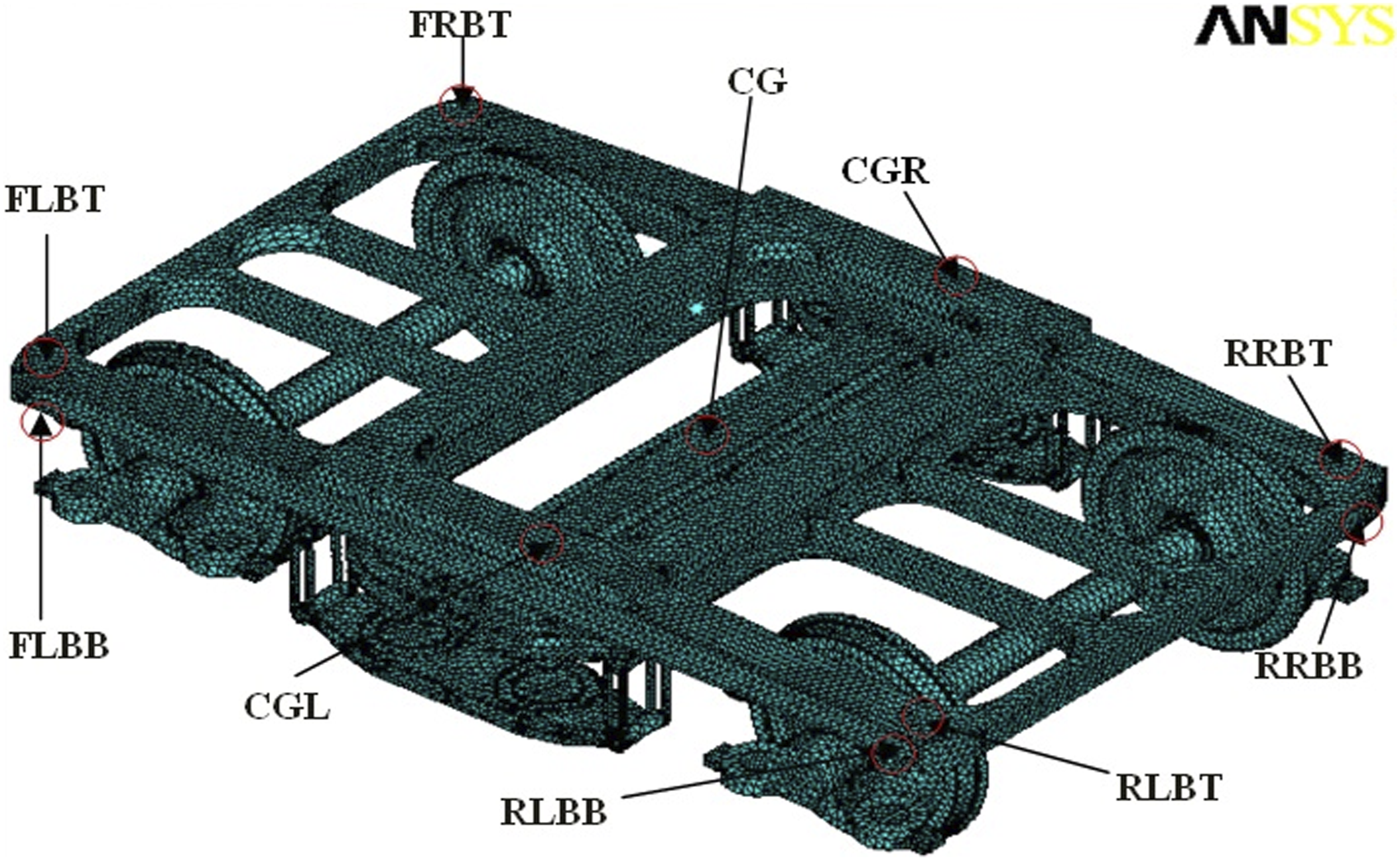

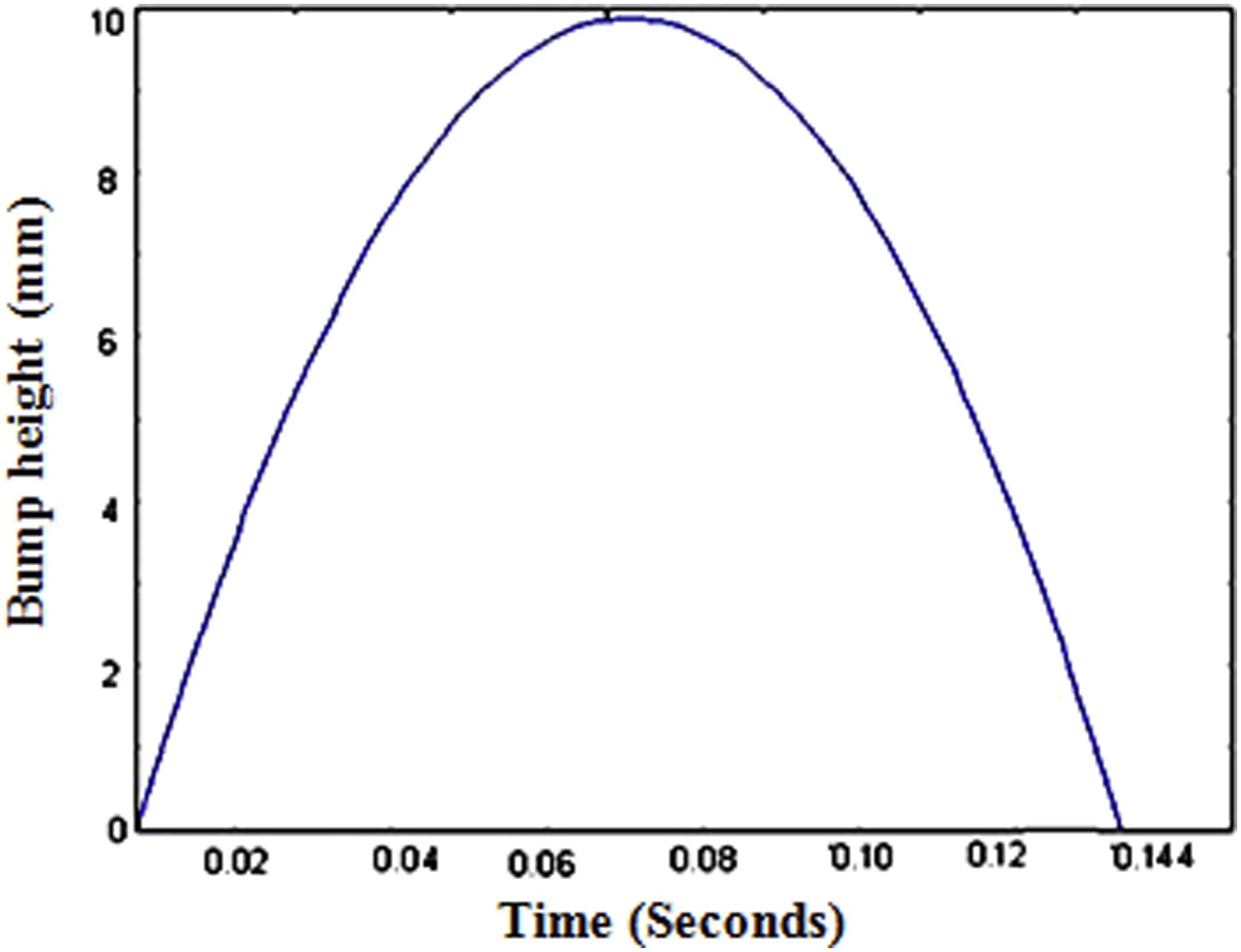
Reference points on the curve of the bump modelled in MATLAB are identified, where the X-axis represents the time range of 0 to 0.144 s and Y-axis represents the wheel vertical displacement with a range of 0 to 10 mm. These values are arranged in two columns of a time history table, where the first column represents the time and the second column represents the vertical displacement of the wheel over the bump. This table in CSV (Comma Separated Values) format is fed as input in ANSYS to the already identified contact points of the four wheels of the bogie.

Transient dynamic analysis of truck

The response of the truck/bogie model subjected to bump excitation at eight-wheel contact points is extracted considering unladen and laden conditions of the truck. Unladen condition does not consider the passenger load on the 6 ton truck; whereas laden condition considers half of the passengers load that is 2.34 tons lumped at the CG of the truck.

Bogie/truck analysis in unladen condition

In the unladen condition, time history plot of vertical displacement response for the CG, CGL and CGR of bogie frame locations is shown in Figure 4.

Figure 4.

Displacement versus time for CG, CGR, and CGL locations of the truck (unladen condition).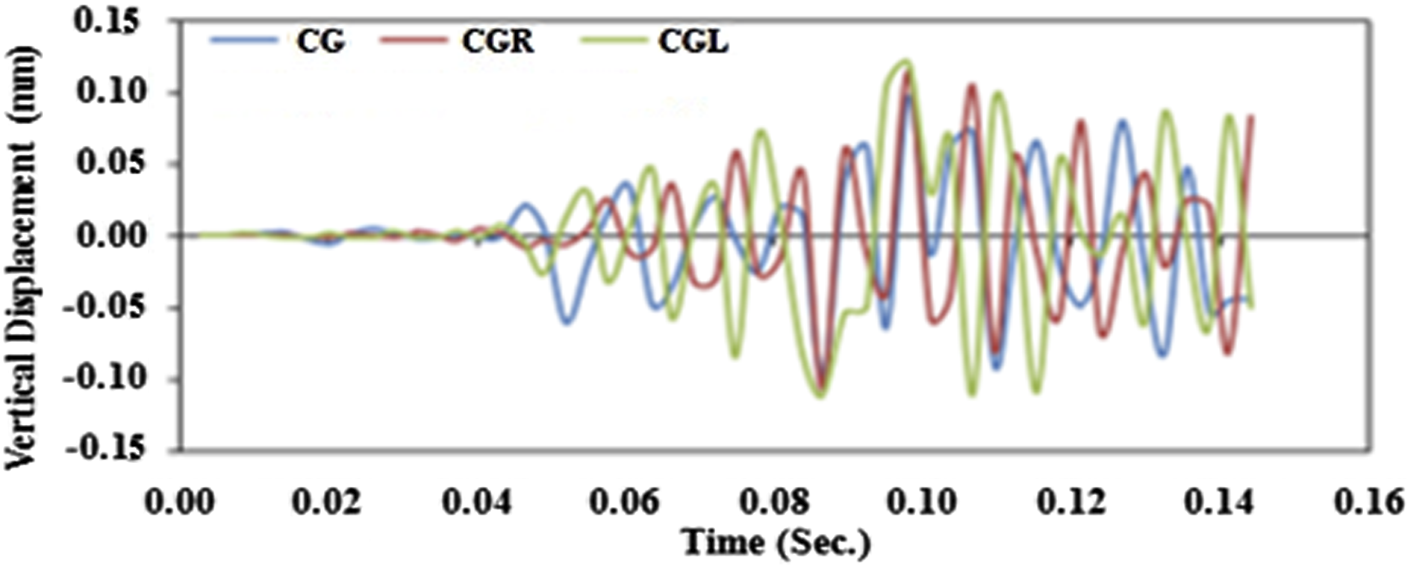

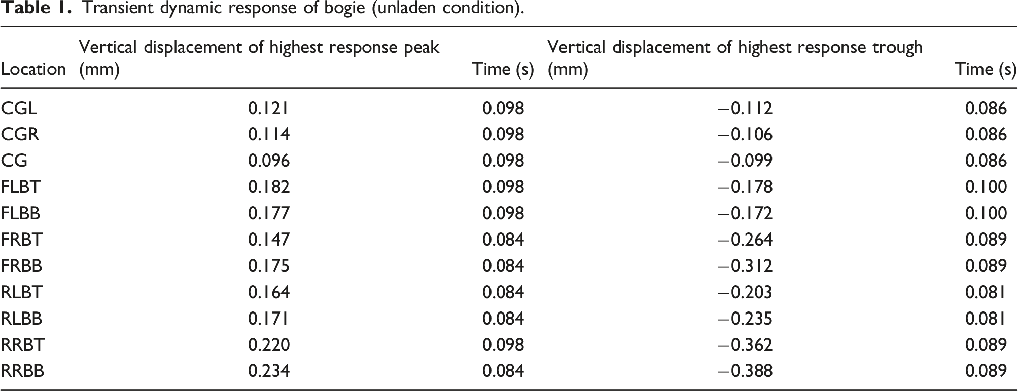
For the first 0.045 s, little disturbance is observed for CG, CGR and CGL as the front wheels may not have reached the obstacle peak.⁴ Once the obstacle has been reached, several peaks and troughs are observed due to the instability of the vehicle once it reaches the bump as per standard literature.^7,8 Vertical displacement response of the front portion of bogie frame at identified locations of the front portion of truck is plotted against time in the time history plot shown in Figures 5 and 6 shows the vertical displacement response of the rear end of the bogie frame.

Figure 5.

Displacement versus time for FLBT, FRBT, FLBB and FLBT locations of the bogie (unladen condition).

Figure 6.

Displacement versus time for RLBT, RRBT, RLBB and RLBT locations of the truck (unladen condition).

The highest peak and trough displacements of the CG, front and rear portions of truck along with corresponding times are tabulated in Table 1. For the truck centre of gravity locations that is CG, CGL, CGR, truck front locations that is FLBT, FLBB, FRBT, FRBB, and truck rear locations namely RLBT, RLBB, RRBT and RRBB; the highest peaks and troughs response is between 0.08 and 0.1 s. This means for the first 0.1 s, the vehicle is ascending the bump and later between 0.1 and 0.144 s, the vehicle descends. The disturbance amplitude of CG is less compared to that of CGR and CGL locations throughout the travel of the vehicle over the bump, as the CGL and CGR locations are away from the centre of gravity¹⁷ and the dynamic forces are relatively unbalanced at these points. From the plots, it can be concluded that the front and rear locations of the unladen truck attain high amplitudes compared to centre of gravity portion as these locations are away from the centre of gravity^4,17 making them susceptible to excitations.

Table 1.

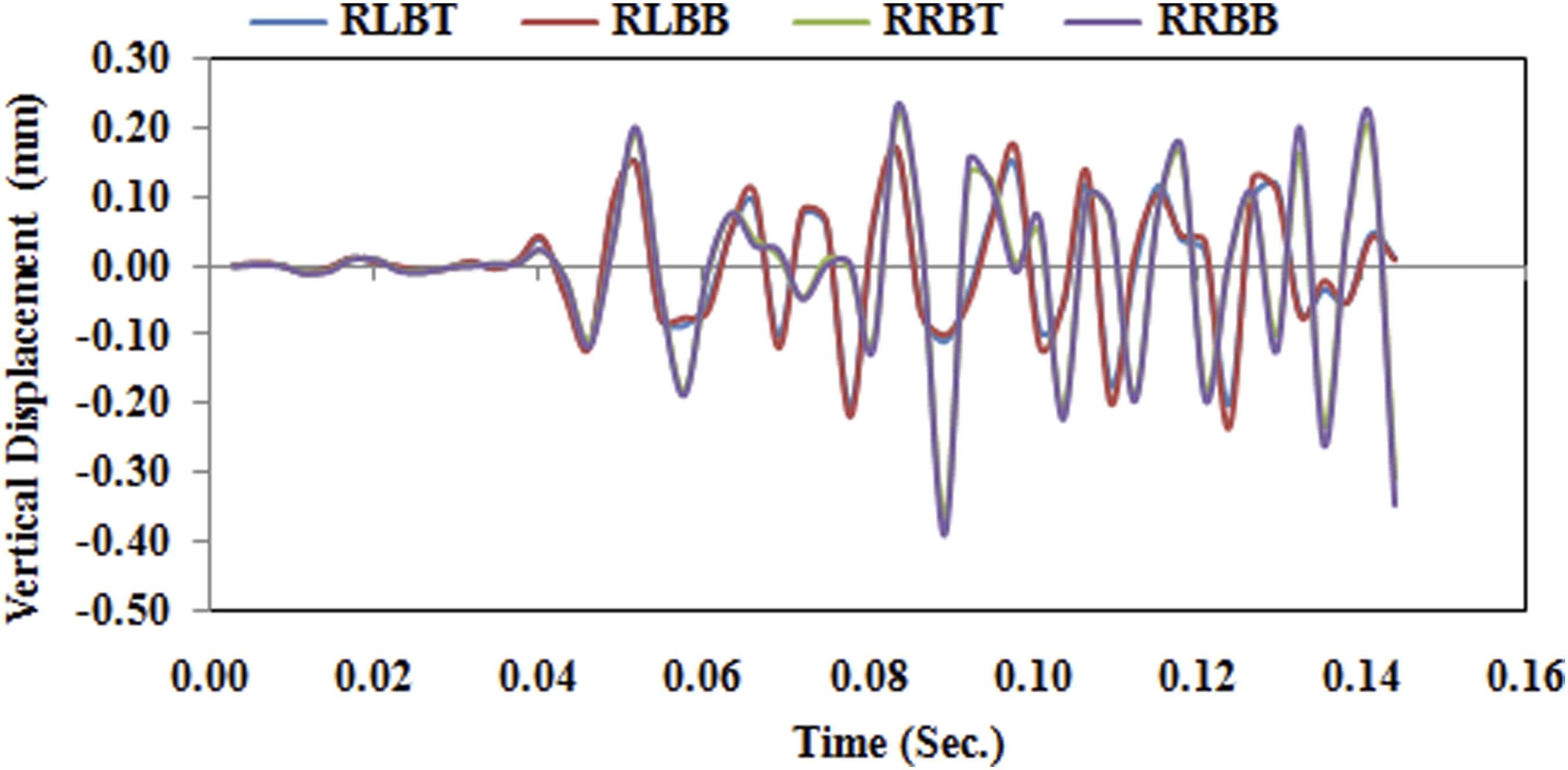
Transient dynamic response of bogie (unladen condition).

Location	Vertical displacement of highest response peak (mm)	Time (s)	Vertical displacement of highest response trough (mm)	Time (s)
CGL	0.121	0.098	−0.112	0.086
CGR	0.114	0.098	−0.106	0.086
CG	0.096	0.098	−0.099	0.086
FLBT	0.182	0.098	−0.178	0.100
FLBB	0.177	0.098	−0.172	0.100
FRBT	0.147	0.084	−0.264	0.089
FRBB	0.175	0.084	−0.312	0.089
RLBT	0.164	0.084	−0.203	0.081
RLBB	0.171	0.084	−0.235	0.081
RRBT	0.220	0.098	−0.362	0.089
RRBB	0.234	0.084	−0.388	0.089

Bogie/truck analysis in laden condition

Considering the passenger load that is 2.34 tons accounting for half of the passengers’ weight in laden condition, the vertical displacement response of the CG, CGL and CGR of bogie frame locations with respect to time is shown in Figure 7. Compared to CGR and CGL, the CG of the laden truck is subjected to lower displacements due to the balanced dynamic forces.⁹

Figure 7.

Displacement versus time for CG, CGR, and CGL locations of the truck (laden condition).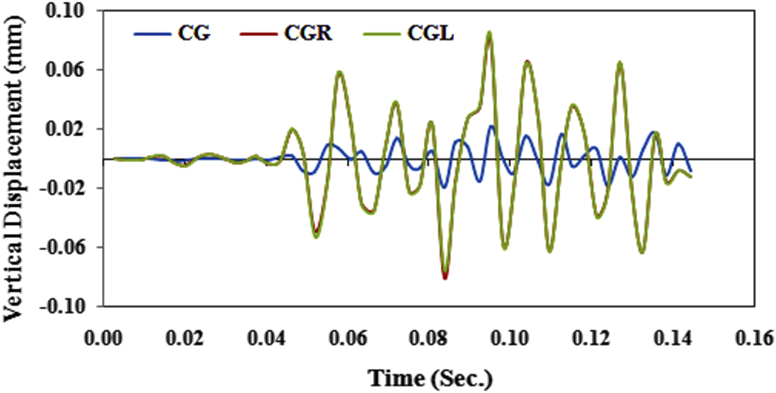

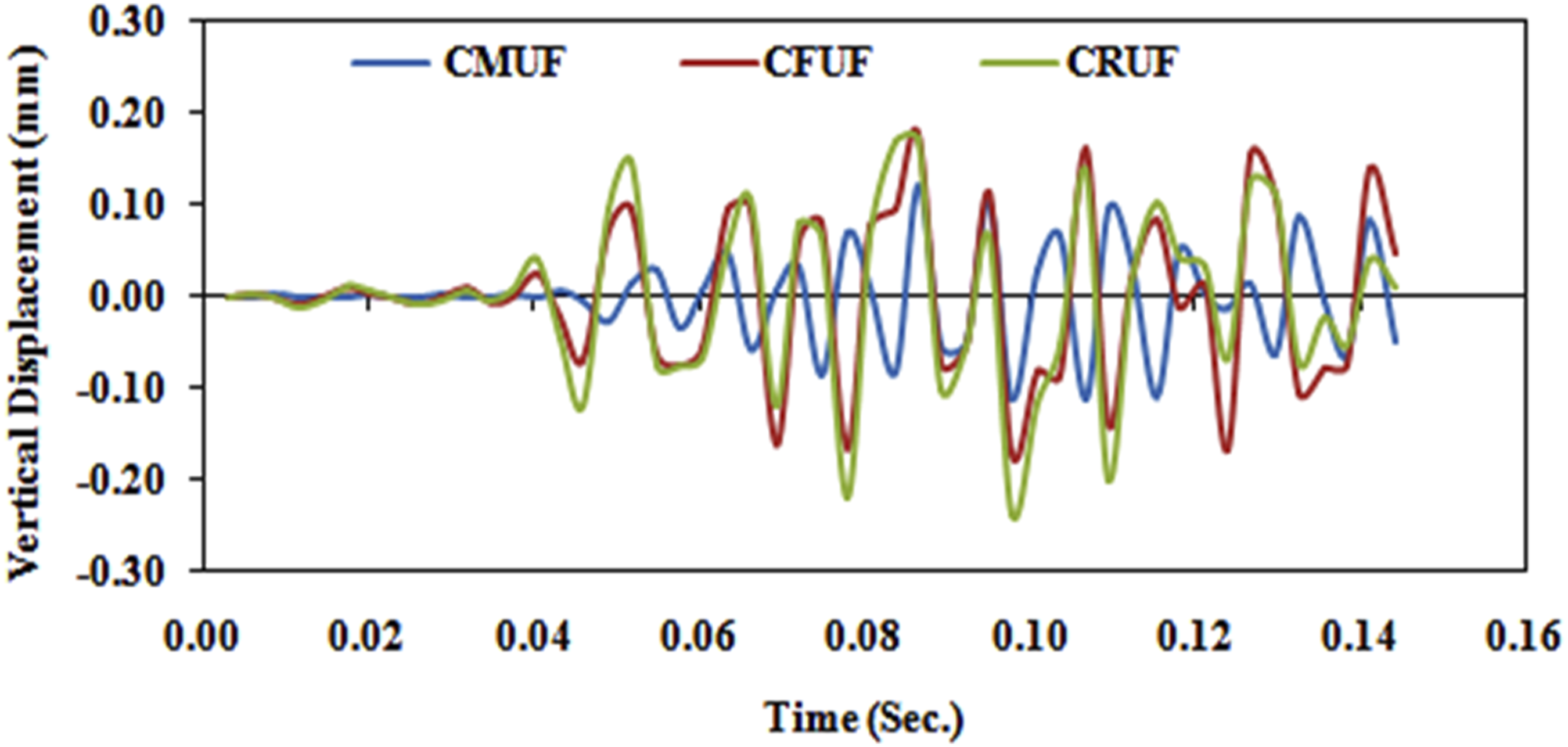
Figure 8 shows the vertical displacement response at FLBB, FLBT, FRBT and FRBB positions in the laden condition. The displacement response pattern of the front left and front right locations are almost similar due to the symmetry about longitudinal axis. The response at RLBT, RLBB, RRBT and RRBB locations in time domain is shown in Figure 9 in the laden condition. The amplitude pattern of these locations shows a similarity with infinitesimal variations due to symmetry about longitudinal axis as per the findings from similar research studies.^4,7,8 The transient response plots from Figures 8–10 show that there is little change in displacement for 0.045 s due to the reason the wheels couldn’t come in contact with the obstacle.^4,7,8 As the wheel comes in contact with the bump and starts crossing, the response is determined from 0.045 s to 0.144 s.

Figure 8.

Displacement versus time for FLBT, FRBT, FLBB and FLBT locations of the bogie (laden condition).

Figure 9.

Displacement versus time for RLBT, RRBT, RLBB and RLBT locations of the bogie (laden condition).

Figure 10.

Displacement versus time for CMUF, CFUF and CRUF locations of the coach underframe (unladen condition).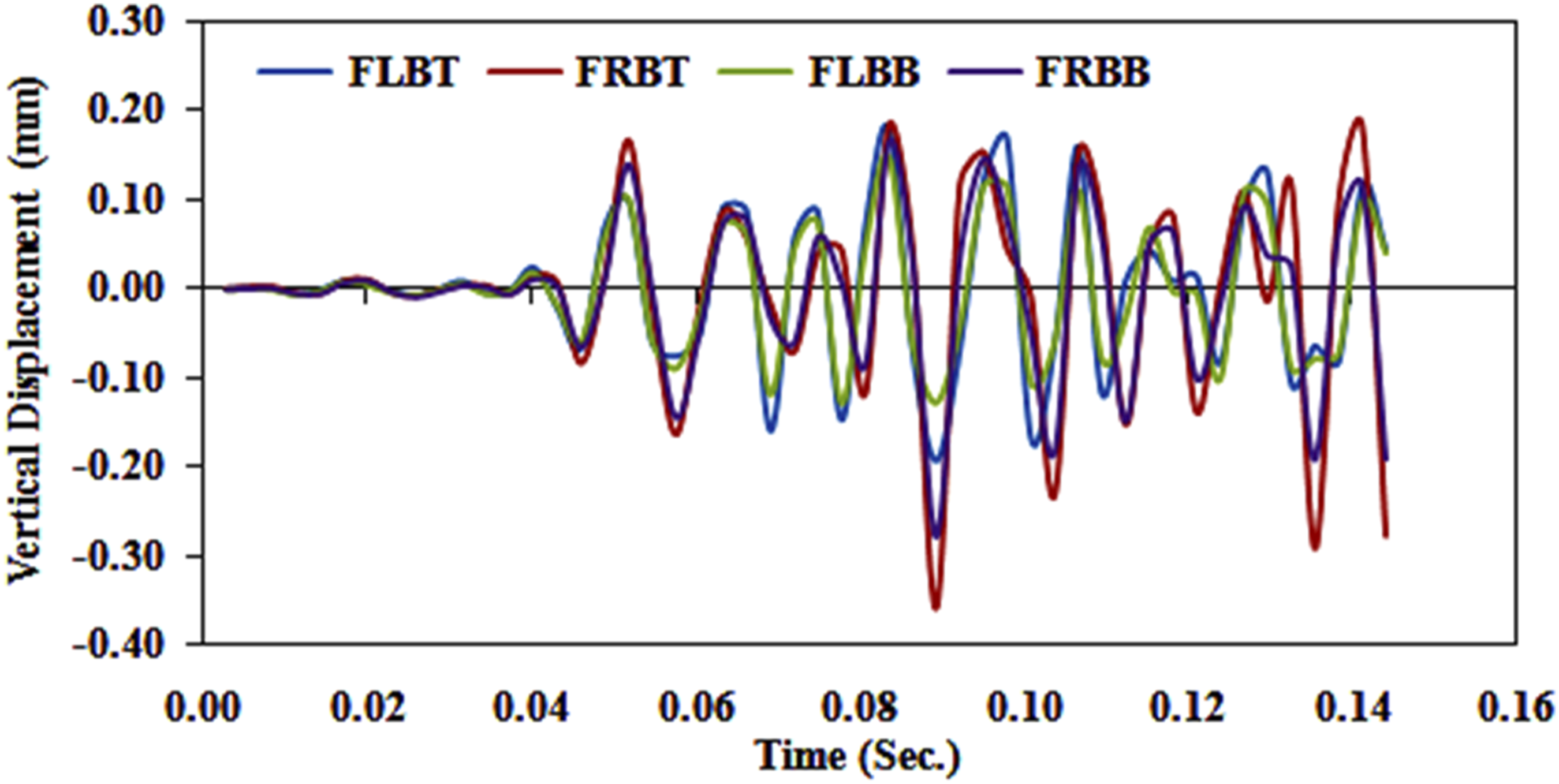

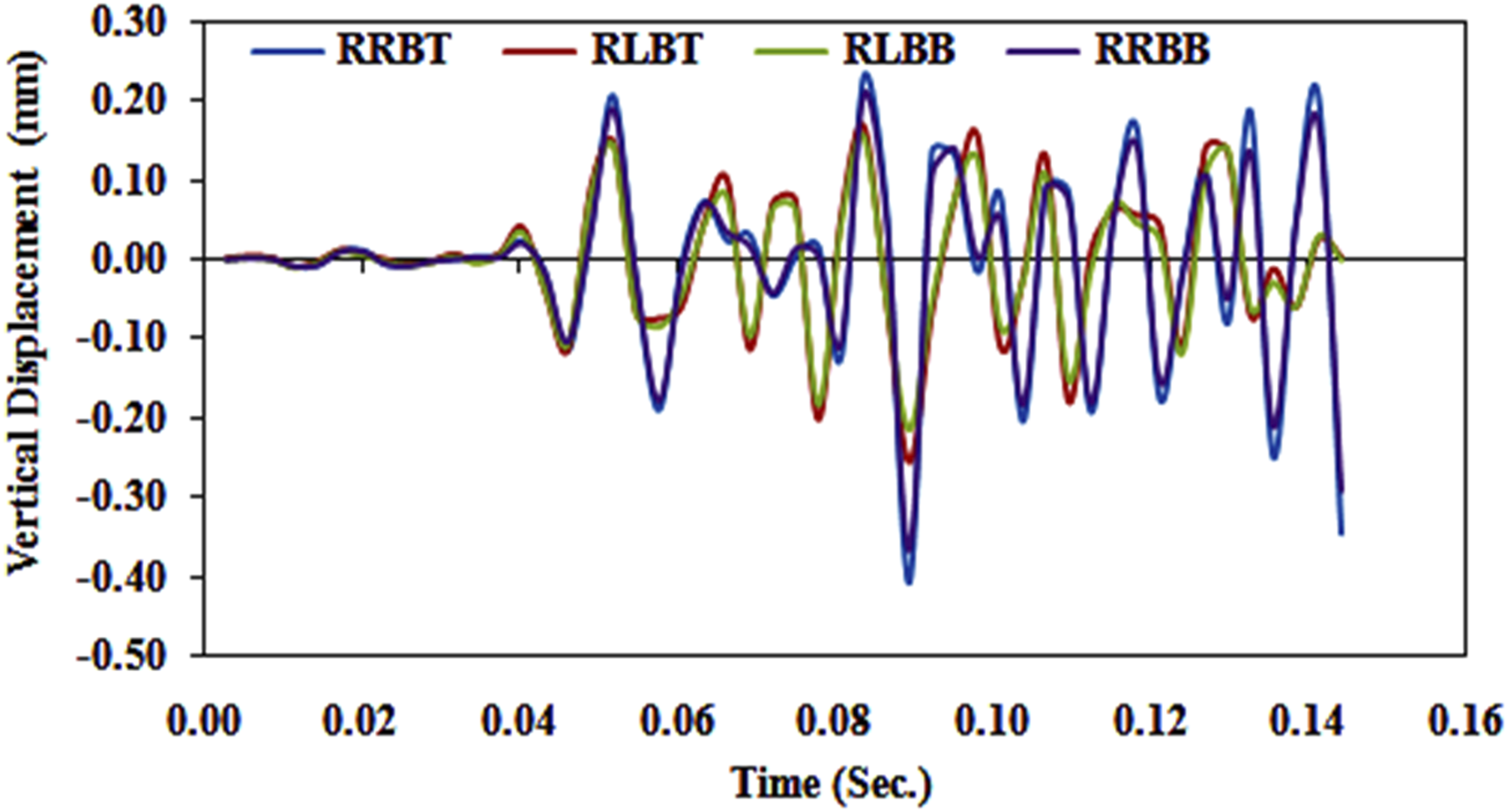
The highest peak and trough displacements of the key locations of the bogie are presented in Table 2. All the highest peaks and troughs for CG, front and rear portions of the laden truck are attained within 0.08 s to 0.1 s. This is due to the ascent of the bogie over the ellipsoidal bump, and between 0.1 s and 0.144 s the truck descends over the bump and hence the displacement response relatively decreases during this period.

Table 2.

Transient dynamic response of bogie frame (laden condition).

Location	Vertical disp. of highest response peak (mm)	Time (s)	Vertical dis. of highest response trough (mm)	Time (s)
CGL	0.083	0.095	−0.075	0.084
CGR	0.081	0.095	−0.080	0.084
CG	0.022	0.095	−0.019	0.084
FLBT	0.128	0.084	−0.193	0.089
FLBB	0.148	0.084	−0.127	0.089
FRBT	0.182	0.084	−0.358	0.089
FRBB	0.166	0.084	−0.278	0.089
RLBT	0.167	0.084	−0.256	0.089
RLBB	0.157	0.084	−0.213	0.089
RRBT	0.230	0.084	−0.407	0.089
RRBB	0.208	0.084	−0.365	0.089

Transient dynamic analysis of locomotive carbody

Time history response of the railway coach model when the wheels of the vehicle cross over the bump in the time period of 0.144 s is extracted in ANSYS Mechanical APDL. The vertical displacement response is extracted and plotted with respect to time for salient locations of the coach underframe and side panel.

Transient dynamic analysis of unladen coach

In unladen condition of the coach, two bottom contact points on each wheel of the front and rear bogies are fed the bump excitation in the form of time history table in ANSYS. The vertical amplitude of the coach underframe front (CFUF), middle (CMUF) and rear (CRUF) locations; as well as the amplitude of coach shell’s left side panel front (FLSP), middle (MLSP), and rear (RLSP) are extracted and plotted with respect to the full time till 0.144 the coach crosses the bump.

Figure 10 is plotted to present the vertical displacement response of the coach underframe when the coach is subjected to the bump excitation. The amplitude of CFUF, CRUF and CMUF locations on the underframe is plotted over the entire period. As CMUF is located at the centre or middle of the underframe where the dynamic loads are more balanced, it shows a relatively lower amplitude than that of CFUF and CRUF.

The displacements observed at prominent locations of the side panel of the coach shell are plotted with respect to the time in Figure 11. The front and rear locations of side panel FLSP and RLSP are near the door openings making these locations more susceptible to excitations resulting in higher amplitudes of disturbances in the entire time frame as presented in standard articles.^4,7,8

Figure 11.

Displacement versus time for MLSP, FLSP and RLSP locations of the coach side panel (unladen condition).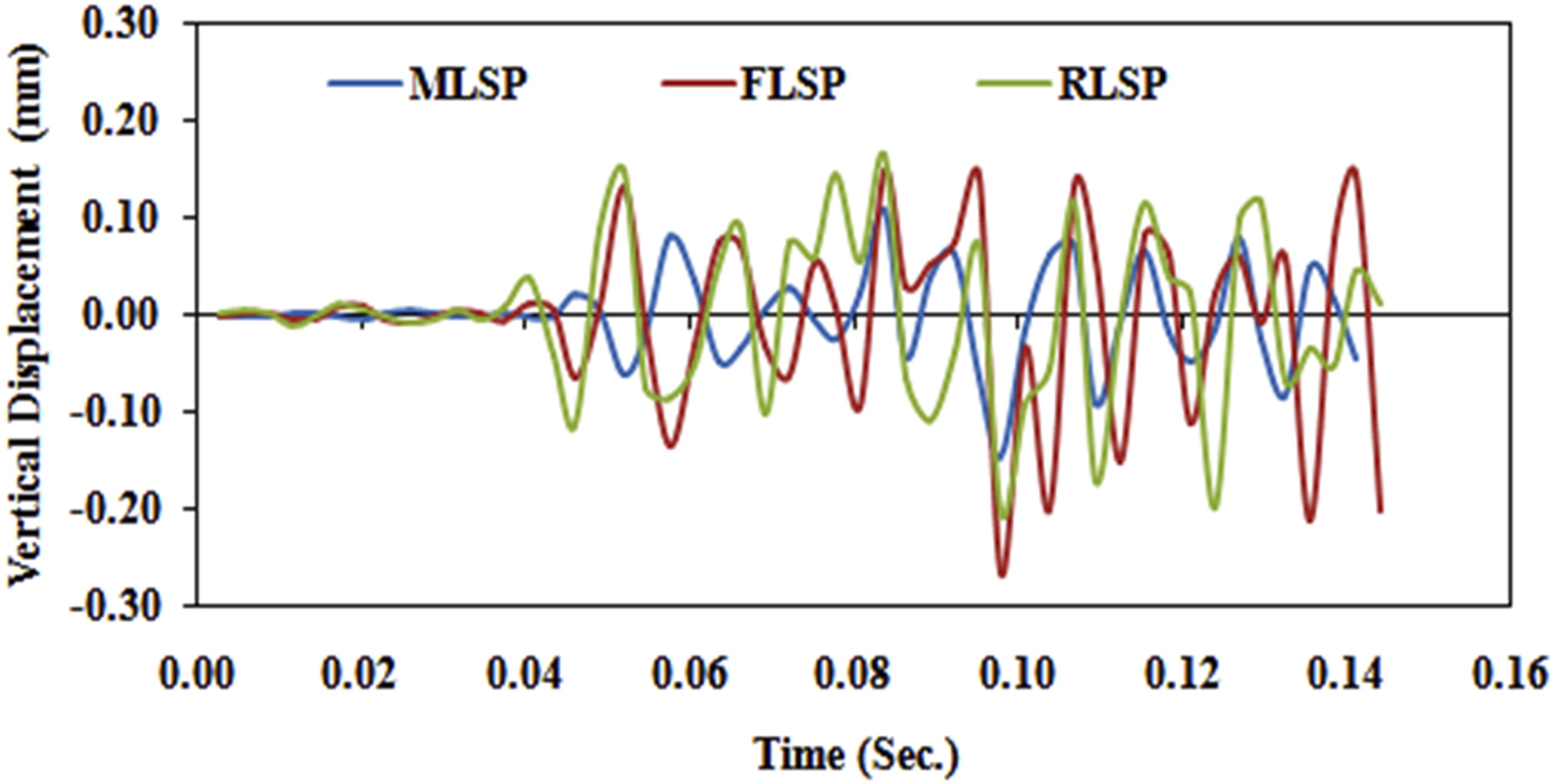

The response to bump excitation of the coach underframe and side panel under the influence of passengers load offers a realistic scenario to study the transient dynamic behavior of the railway coach. Total 72 passengers load of 4.68 tons is lumped at the CG of the coach FE model using mass coupling and constraint equations in ANSYS Mechanical APDL.

The disturbance amplitudes of the underframe locations CFUF, CRUF and CMUF are plotted in Figure 12 in the entire period. It is observed that the front and rear locations of the underframe, that is CFUF and CRUF are subjected to higher displacements than that of the middle location CMUF due to the extended distance from the centre of gravity and unbalanced distribution of dynamic forces.

Figure 12.

Displacement versus time for CMUF, CFUF and CRUF locations of the coach underframe (laden condition).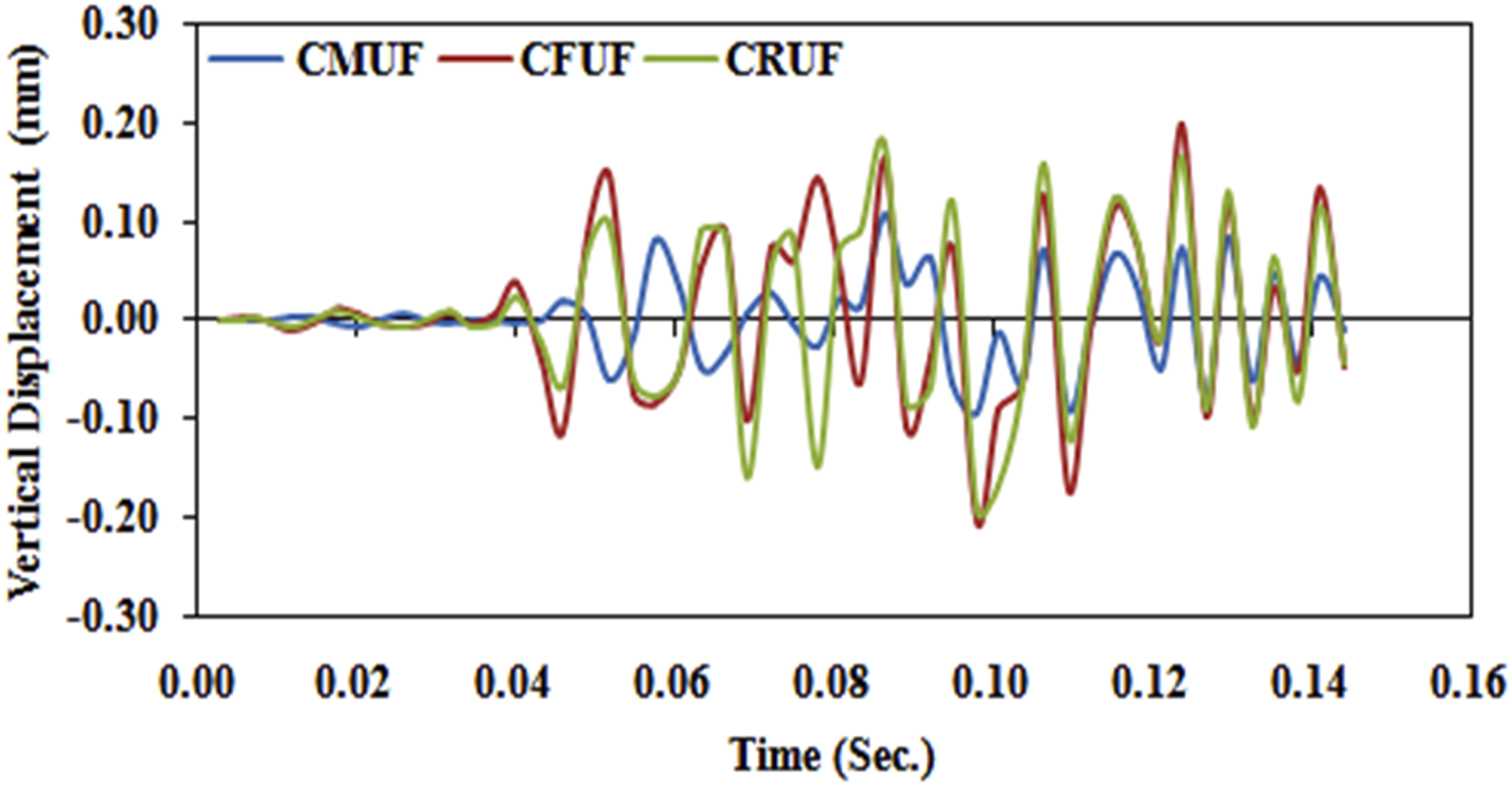

The response of the side panel locations to bump excitation in the laden condition of the coach is presented in Figure 13. The plot indicates that the middle portion of the side panel has lower vertical displacements compared to that front and rear locations of coach shell in the entire duration of 1.44 s. The middle location of side panel MLSP lies closer to the centre of gravity due to which the disturbance amplitude is relatively less.

Figure 13.

Displacement versus time for MLSP, FLSP and RLSP locations of the coach side panel (laden condition).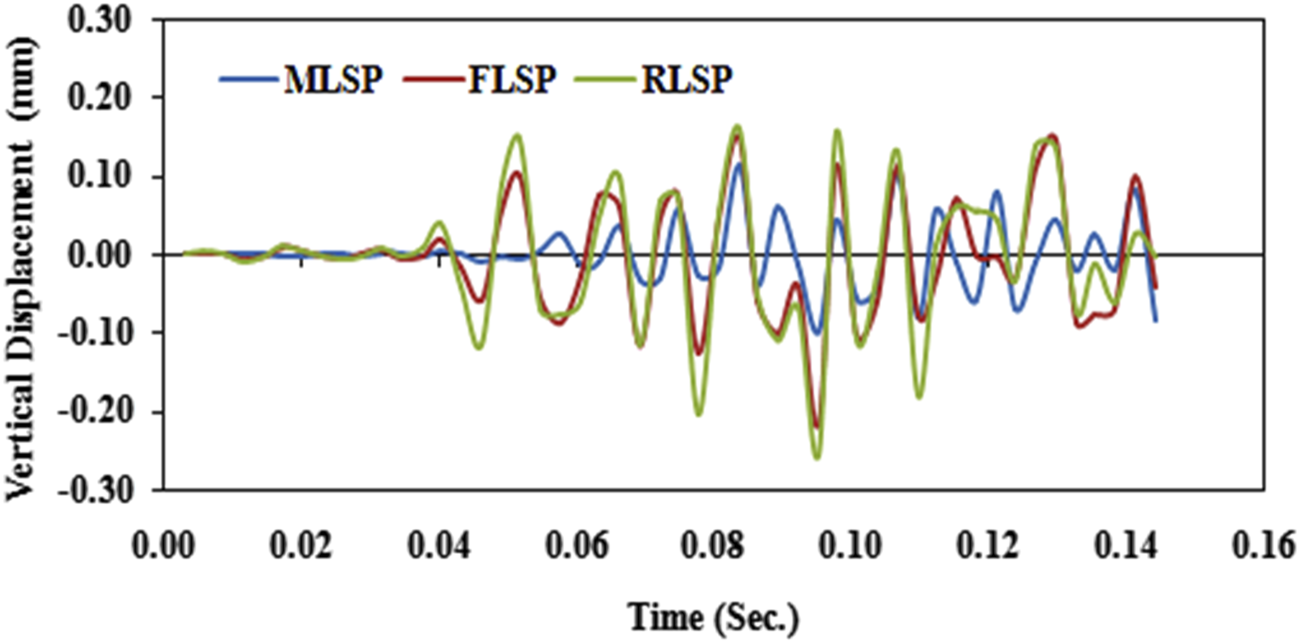

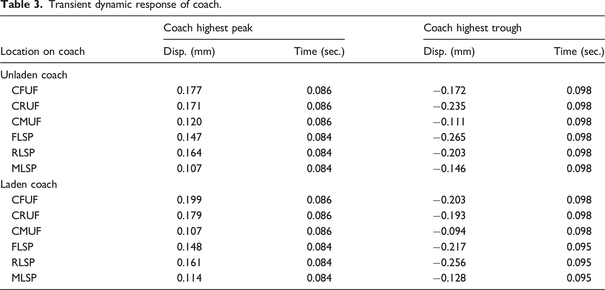
Table 3 presents the highest response peaks and troughs of the coach underframe and side panel under unladen and laden conditions. From the plots and results obtained, it can be concluded that the coach shows little variations in displacements till 0.045 s as it does not reach the obstacle specified in the literature,⁴ later the amplitude of disturbances increases between 0.045 s and 0.144 s. The highest amplitudes of peaks and troughs are observed between 0.08 s and 0.1 s, indicating the ascending vehicle over the ellipsoidal bump. Beyond 0.1 s till 0.144 s the vehicle descends and hence the amplitudes of peaks and troughs come down.

Table 3.

Transient dynamic response of coach.

Location on coach	Coach highest peak		Coach highest trough
Location on coach	Disp. (mm)	Time (sec.)	Disp. (mm)	Time (sec.)
Unladen coach
CFUF	0.177	0.086	−0.172	0.098
CRUF	0.171	0.086	−0.235	0.098
CMUF	0.120	0.086	−0.111	0.098
FLSP	0.147	0.084	−0.265	0.098
RLSP	0.164	0.084	−0.203	0.098
MLSP	0.107	0.084	−0.146	0.098
Laden coach
CFUF	0.199	0.086	−0.203	0.098
CRUF	0.179	0.086	−0.193	0.098
CMUF	0.107	0.086	−0.094	0.098
FLSP	0.148	0.084	−0.217	0.095
RLSP	0.161	0.084	−0.256	0.095
MLSP	0.114	0.084	−0.128	0.095

Random track inputs measured using track recording car (TRC)

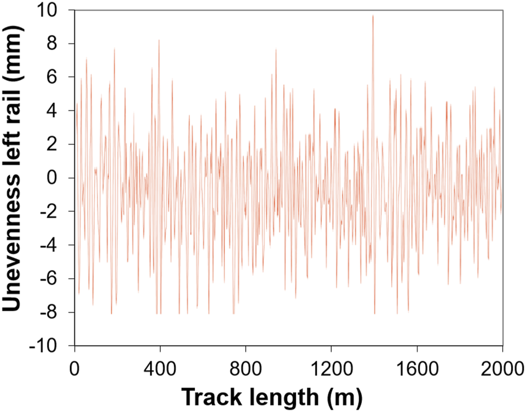
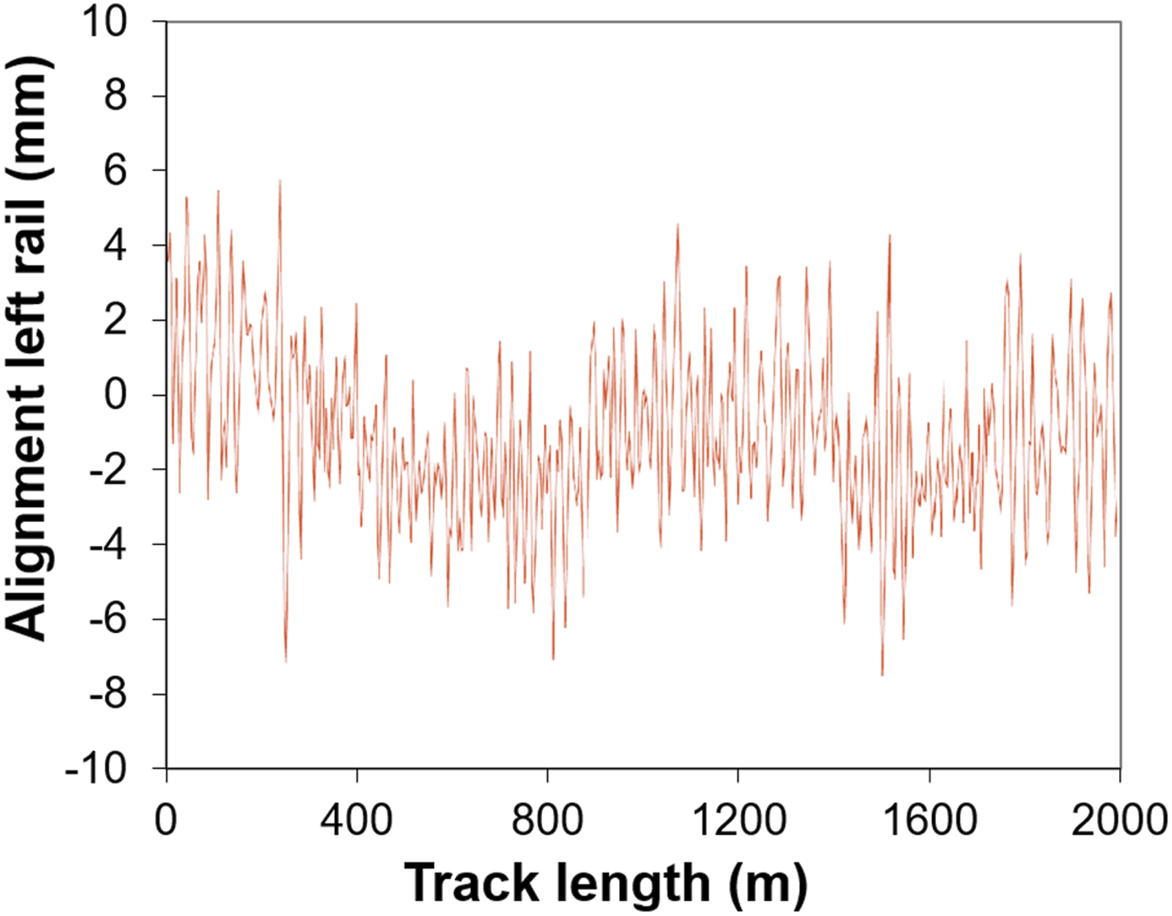
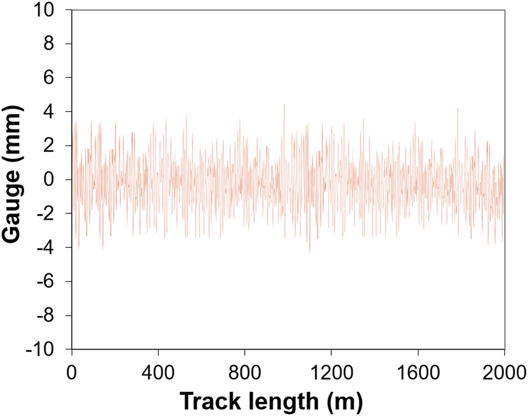
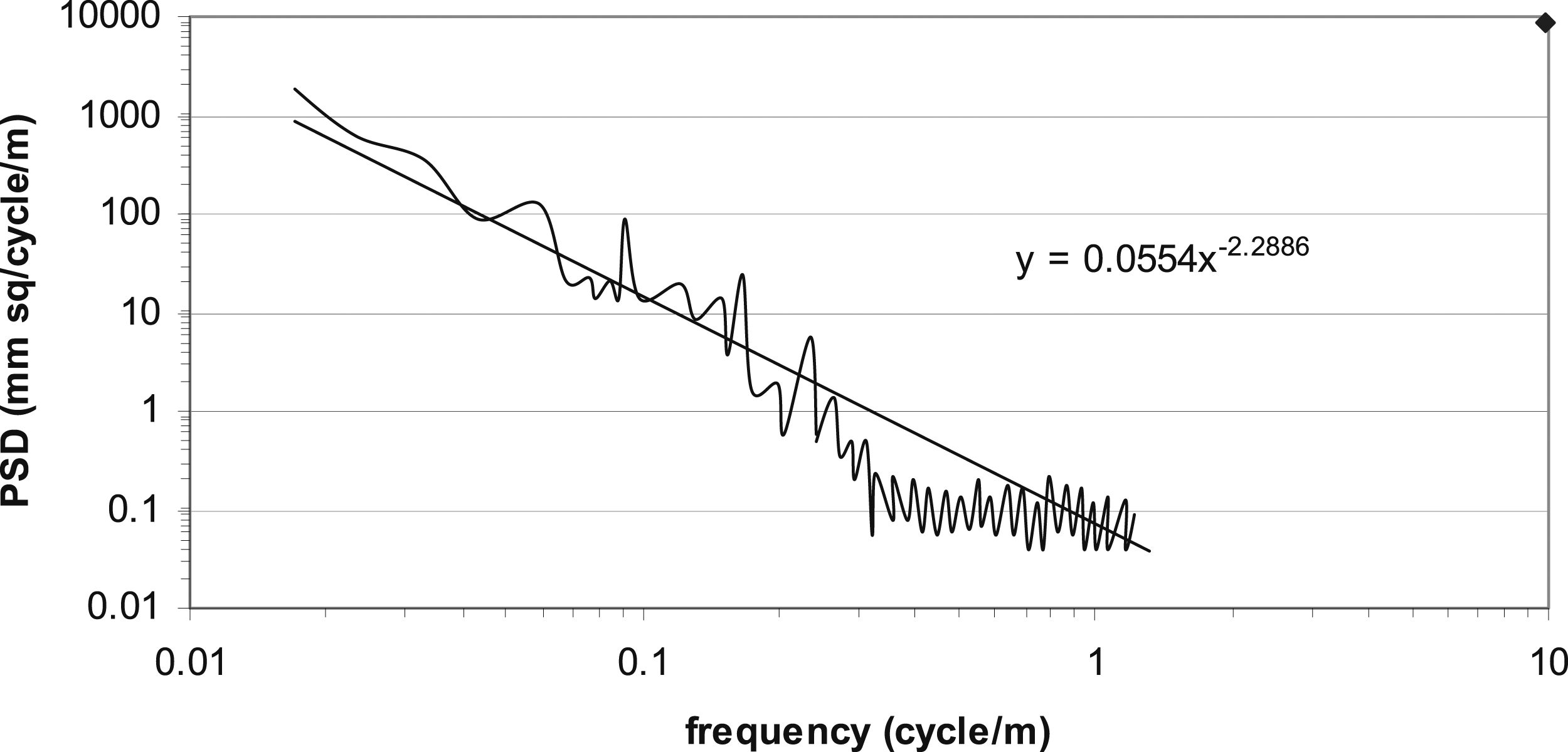
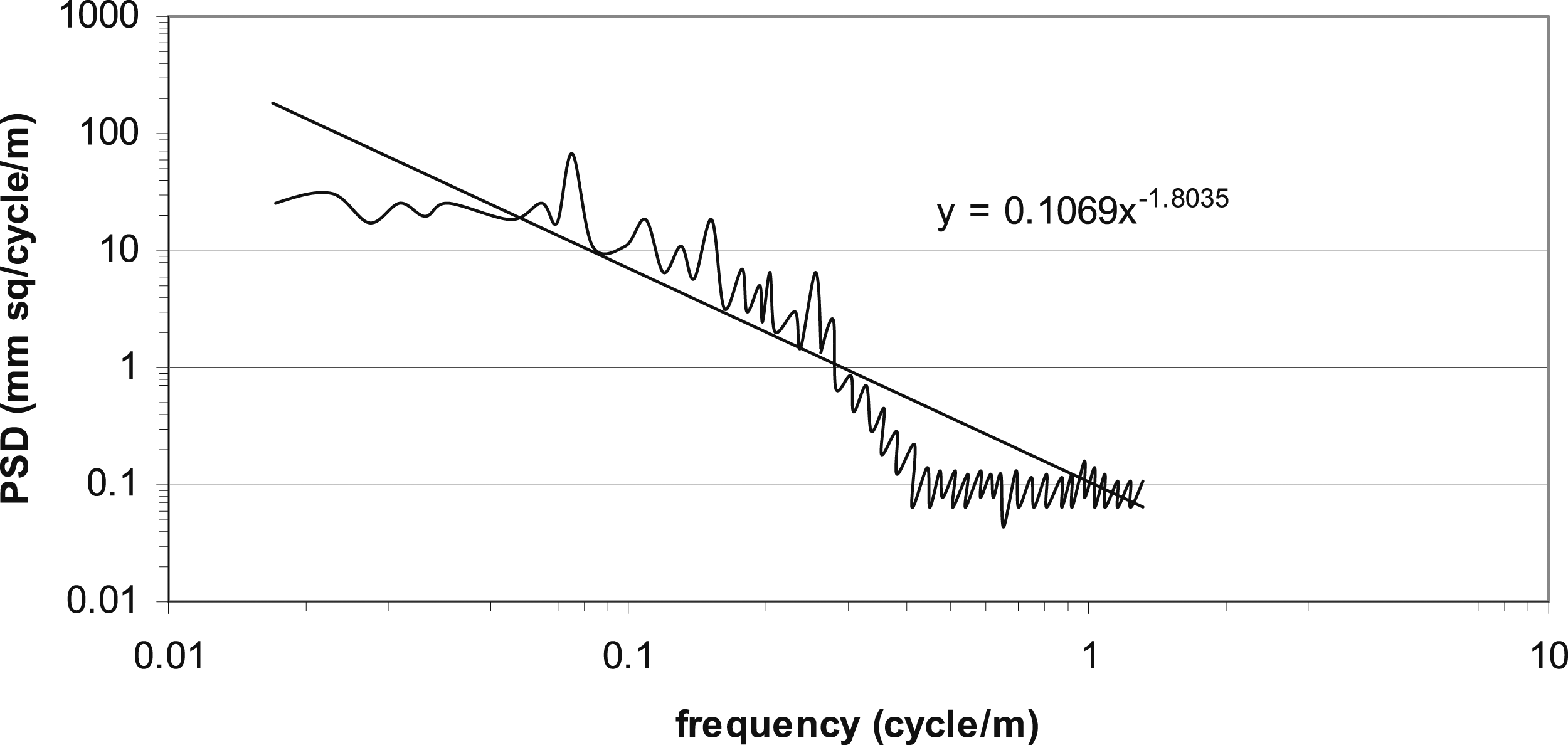
Indian railway uses TRC to evaluate the track undulations in real-time history. The measured track irregularities are unevenness (left and right rail), alignment (left and right rail), cross-level, gauge etc. The track geometry variations which largely affect the rail vehicle behavior are measured by TRC using either the chord offset principle or the inertial principle. An inside view of TRC with track geometry measurement system is shown in Figure 14. Figures 15–17 show the unevenness of left rail, variation in alignment left rail and variation in track gauge respectively.

Figure 14.

Track geometry measurement system of TRC.

Figure 15.

Unevenness of left rail.

Figure 16.

Variation in alignment: left rail.

Figure 17.

Variation in track gauge.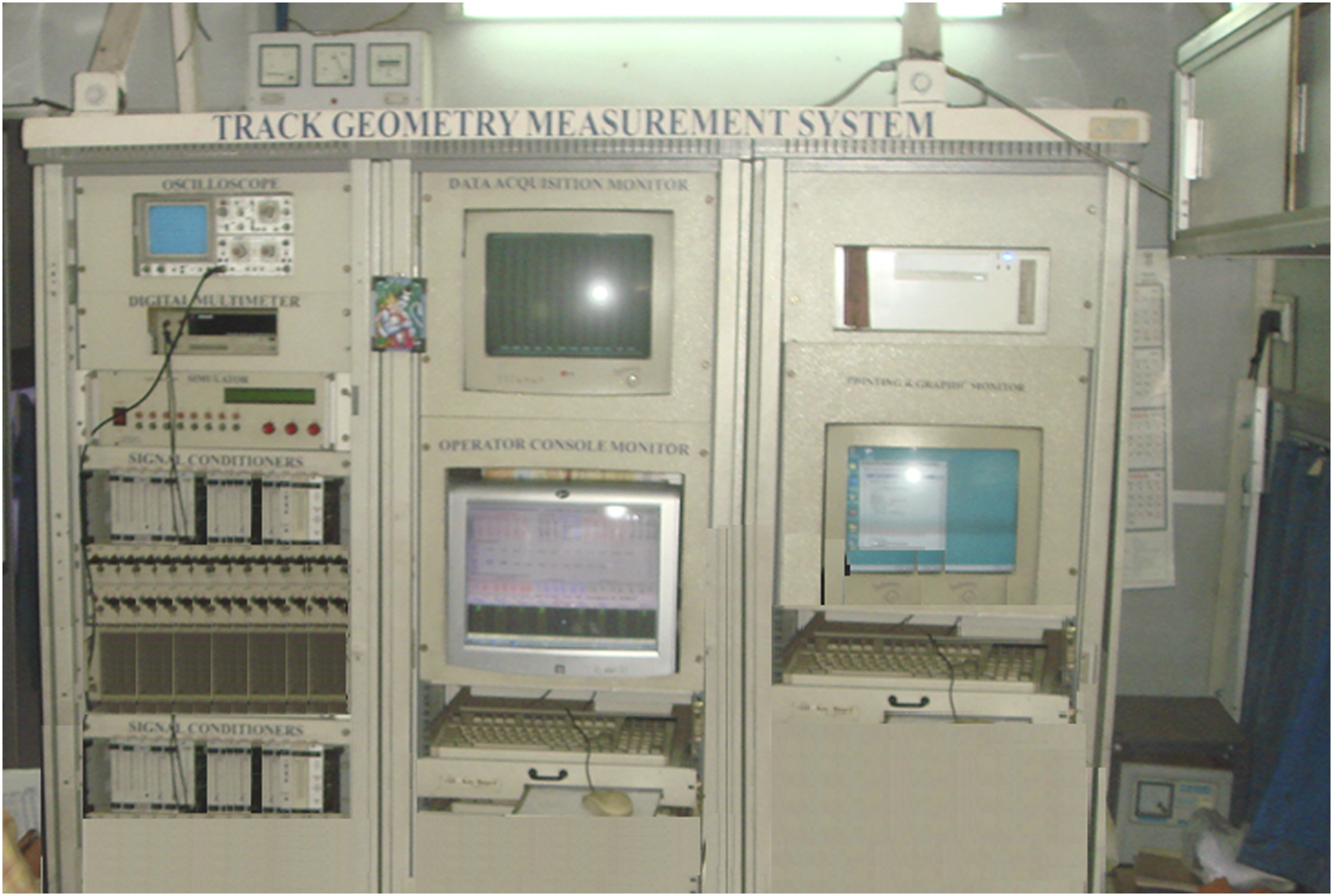

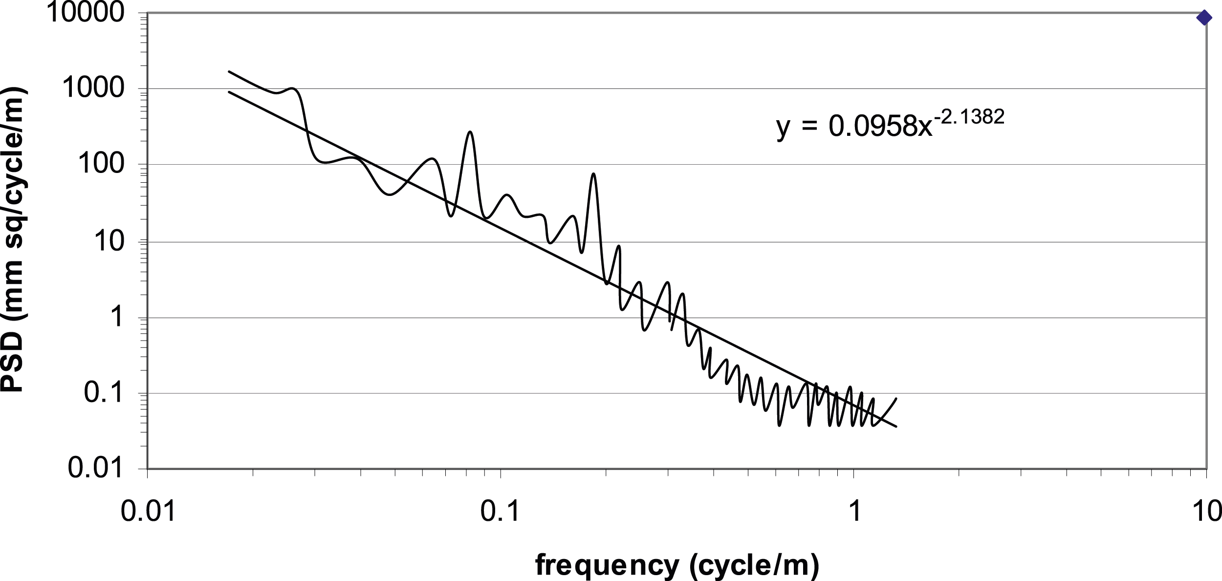
These track geometry variations are represented as PSD using Fast Fourier Transformation and are expressed in the following form as a function of spatial frequency $Ω$ .

S^{z, y} (Ω) = C_{S P} {(Ω)}^{- N}

(2)

C_{S P}

is an empirical constant, and N characterizes the rate at which amplitude decreases with wavelength or frequency. The larger the value of N, the amplitude decreases speedily. PSD variations of unevenness (left), alignment (left) and track gauge are shown in Figures 18–20 respectively.

Figure 18.

PSD variation of unevenness of left rail.

Figure 19.

PSD variation of alignment of left rail.

Figure 20.

PSD variation of track gauge variations.

Rigid body model of railway vehicle

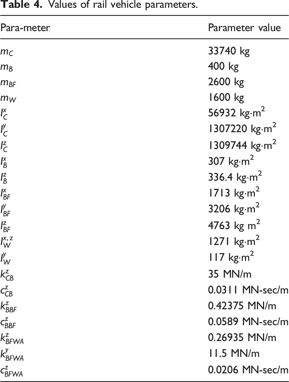
Figure 21 shows the analytical model of railway vehicle formulated assigning 37 Degrees of Freedom to the main rigid bodies that is carbody (vertical, lateral, roll, pitch and yaw), two bolsters (vertical, lateral, and roll), two bogie frames (vertical, lateral, roll, pitch and yaw), and the four-wheel axles (vertical, lateral, roll, and yaw). Linear suspension is assumed between these rigid bodies and parameter values are obtained from Research Design Standards Organisation, Lucknow, India and are listed in Table 4.

Figure 21.

Rigid body model of railway vehicle.

Table 4.

Values of rail vehicle parameters.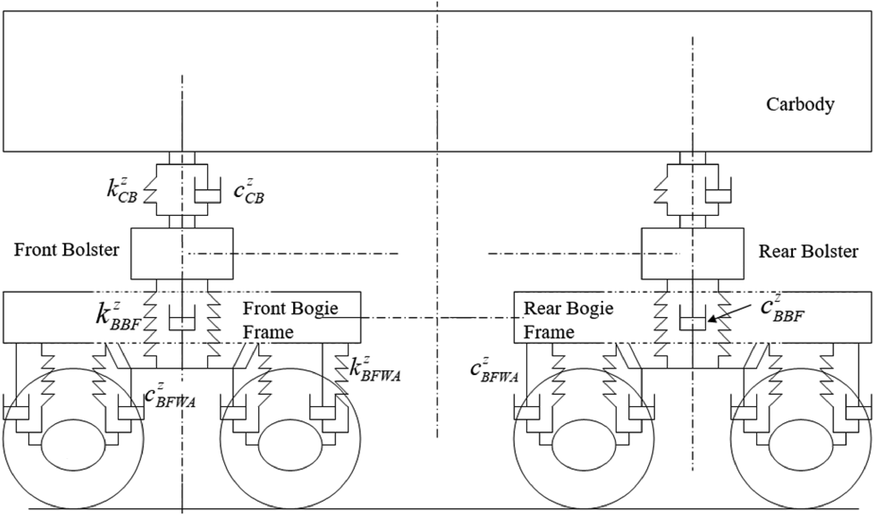

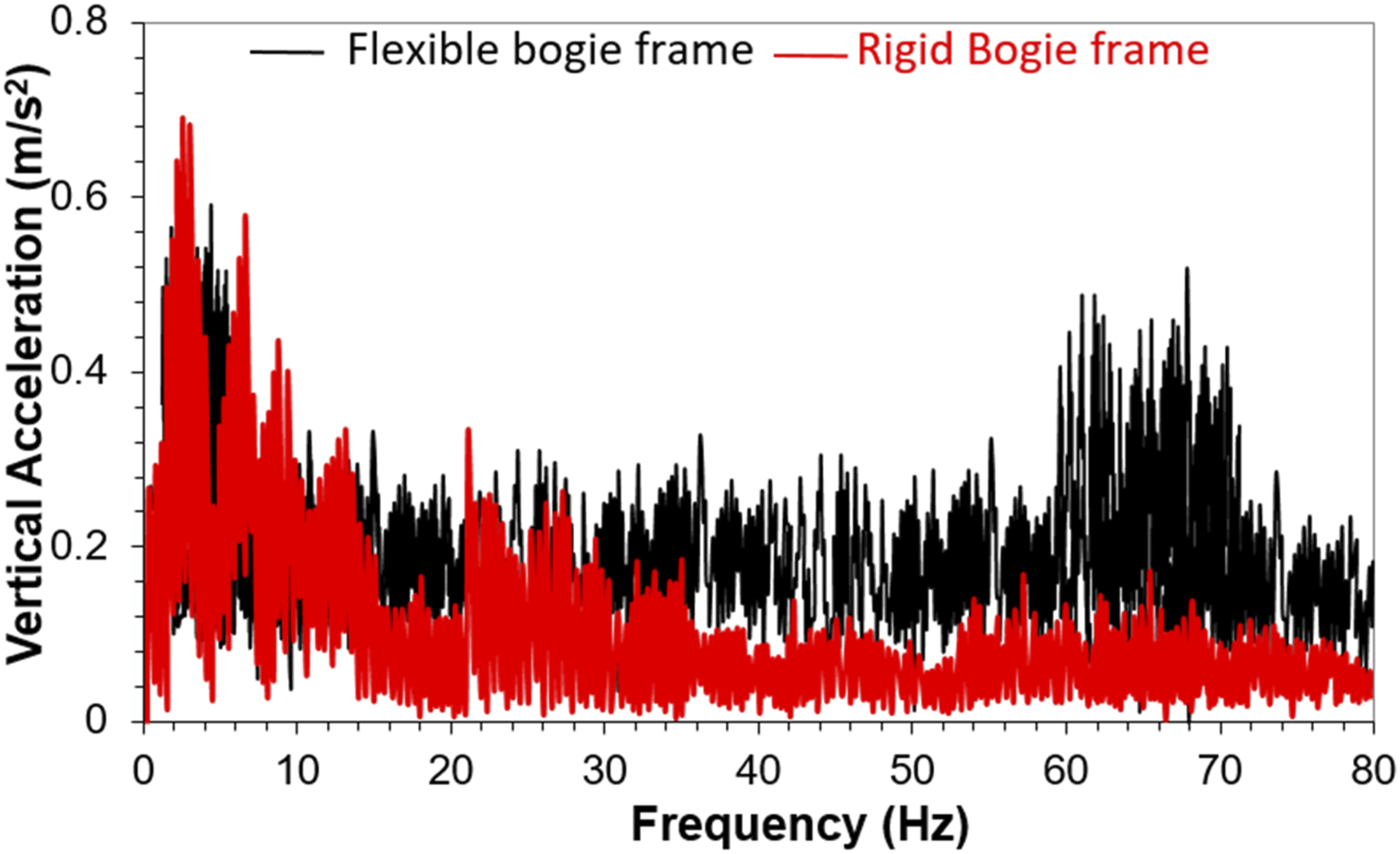
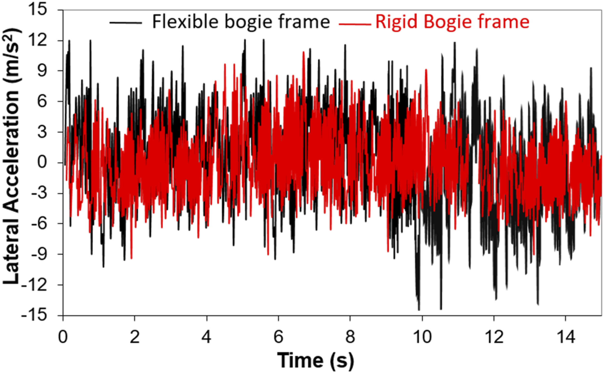
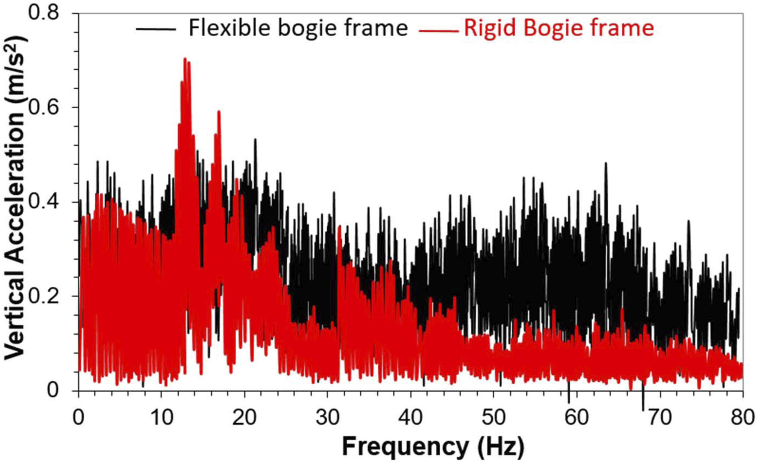
Para-meter	Parameter value
$m_{C}$	33740 kg
$m_{B}$	400 kg
$m_{B F}$	2600 kg
$m_{W}$	1600 kg
$I_{C}^{x}$	56932 kg·m²
$I_{C}^{y}$	1307220 kg·m²
$I_{C}^{z}$	1309744 kg·m²
$I_{B}^{x}$	307 kg·m²
$I_{B}^{z}$	336.4 kg·m²
$I_{B F}^{x}$	1713 kg·m²
$I_{B F}^{y}$	3206 kg·m²
$I_{B F}^{z}$	4763 kg m²
$I_{W}^{x, z}$	1271 kg·m²
$I_{W}^{y}$	117 kg·m²
$k_{C B}^{z}$	35 MN/m
$c_{C B}^{z}$	0.0311 MN-sec/m
$k_{B B F}^{z}$	0.42375 MN/m
$c_{B B F}^{z}$	0.0589 MN-sec/m
$k_{B F W A}^{z}$	0.26935 MN/m
$k_{B F W A}^{y}$	11.5 MN/m
$c_{B F W A}^{z}$	0.0206 MN-sec/m

The formulated rigid body model is subjected to PSD random inputs as obtained from TRC. The same inputs provided to flexible FM model are the results of vertical and lateral accelerations of bogie frame centre are plotted in time and frequency domain and are shown in Figures 22–25. The time domain analysis of vertical and lateral acceleration of bogie frame suggests that with rigid body analysis the acceleration values obtained are in a lower range as compared with the same obtained from finite element flexible bogie frame analysis. The frequency domain analysis of vertical and lateral acceleration suggests that acceleration values are compatible in lower frequency ranges up to nearly 10 Hz. Beyond 10 Hz, the acceleration values obtained with finite element analysis are much higher as compared with the same obtained with the rigid body analysis. Results obtained from Finite Element models and analytical models may not exactly similar because the two approaches have their own limitations. Finite Element models have lack of physical replicas of spring suspensions, since the suspension systems are modelled using COMBIN element in FEA. With Finite Element models geometrical features in the vehicle that are insignificant from load bearing point of view are neglected in vehicle modeling and hence their response is also not determined. Rigid body model considers the contact patch is as Hertzian ellipse. The creep forces are considered as linear function of creepage that is wheel axle set displacements and wheel axle set velocities. In actual the creep forces are non-linear functions of wheel-axle set displacements and wheel-axle set velocities. Rigid body model considers the suspension forces are assumed as linear function of displacement and velocities within the range of their travel. In actual practice the piecewise linear theory is applicable considering the actual travel of the suspension elements. Due to these limitations with the two methods results may be different and a few discrepancies are possible.

Figure 22.

Vertical acceleration of bogie frame centre (time domain).

Figure 23.

Vertical acceleration of bogie frame centre (frequency domain).

Figure 24.

Lateral acceleration of bogie frame centre (time domain).

Figure 25.

Lateral acceleration of bogie frame centre (frequency domain).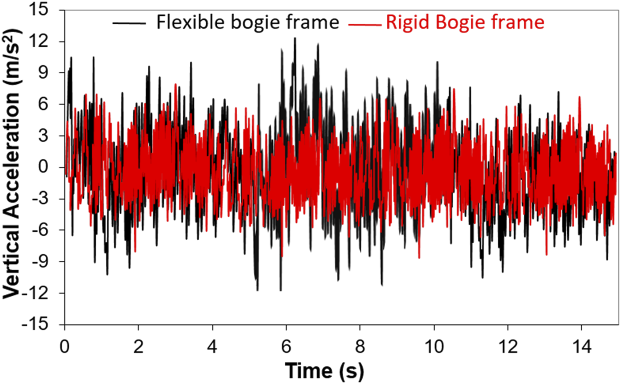

Conclusions

The time domain method is effectively used to analyze the vehicle body’s behavior subjected to real-time input excitations⁴ as the vehicle traverses a semi-circular bump. The results obtained from the present analysis suggest that when the train at 100 kmph crosses the ellipsoidal bump the response at the truck front and rear portions is higher than its centre of gravity location. The centre or middle portion of carbody underframe and side panel show a lower amplitude of disturbances over the entire period due to balanced dynamic forces near centre of gravity. Variations in response patterns under unladen and laden conditions of the truck, as well as for the carbody respectively indicate that the passenger weight has a significant effect on the transient dynamic response supported by literature.^3,4,17 The results indicate that for initial 0.045 s the vehicle does not reach the bump, then till 0.1 s the vehicle ascends the bump and between 0.1 s and 0.144 s the vehicle descends. From the results of transient dynamic analysis, it is concluded that the front and rear portions of the laden truck are subjected to disturbances with higher amplitude compared to that of centre of gravity locations. Since the front and rear portions of the truck are at an extended distance from the CG of the truck those locations are more vulnerable to bump excitation. The front and rear locations of carbody underframe and side panel are subjected to higher displacement values compared to that of the middle locations which are in the vicinity of centre of gravity of the carbody. The comparative analysis of finite element and rigid body analysis suggests that the two approaches are compatible in the lower frequency range up to 10 Hz frequency. Beyond that, the acceleration values differ significantly.

Footnotes

Author contributions

Dr Rakesh Chandmal Sharma: Simulation, Results, Dr Srihari Palli: Modelling, Dr D Loknadham: Simulation, Dr Sunil Kumar Sharma: Simulation, Revision, Dr Ashwini Sharma: Simulation, Revision, Dr Ashwani Kharola: Simulation, Dr Neeraj Sharma, Simulation.

Declaration of conflicting interests

The author(s) declared no potential conflicts of interest with respect to the research, authorship, and/or publication of this article.

Funding

The author(s) received no financial support for the research, authorship, and/or publication of this article.

ORCID iDs

Rakesh Chandmal Sharma

Srihari Palli

Sunil Kumar Sharma

Appendix

References

Popp

Kaiser

Kruse

. System dynamics of railway vehicles and track. Arch Appl Mech 2003; 72(11): 949–961.

Popp

Knothe

Pöpper

. System dynamics and long-term behaviour of railway vehicles, track and subgrade: report on the DFG priority programme in Germany and subsequent research. Veh Syst Dyn 2005; 43(6–7): 485–521.

Pombo

Ambrósio

. Dynamic analysis of a railway vehicle in real operation conditions using a new wheel-rail contact detection model. Int J Veh Syst Model Test. 2005; 1(1–3): 79–105.

Ramji

Goel

Rao

, et al. Dynamic behaviour of railway coach and bogie frame using finite element analysis. J Inst Eng, Part MC, Mech Engg Div 2007; 87(4): 7–17.

Sharma

. Combined multi-body-system and finite element analysis of a rail locomotive crashworthiness. Int J Veh Struct Syst 2020; 12: 428–435.

Bhardawaj

Sharma

. Analysis of frontal car crash characteristics using ANSYS. Mater Today Proc 2020; 25: 898–902.

Mazilu

. An analysis of bogie hunting instability. UPB Scien Bull Series D: Mech Eng 2009; 71(2): 64–78.

Abood

Khan

. Hunting phenomenon study of railway conventional truck on tangent tracks due to change in rail wheel geometry. J Eng Sci Technol 2011; 6(2): 146–160.

Sharma

. Ride, eigenvalue and stability analysis of three-wheel vehicle using Lagrangian dynamics. Int J Veh Noise Vib 2017; 13: 13–25.

10.

Bhardawaj

Sharma

. Development in the modeling of rail vehicle system for the analysis of lateral stability. Mater Today Proc 2020; 25: 610–619.

11.

Sharma

Lee

. Effect of rail vehicle–track coupled dynamics on fatigue failure of coil spring in a suspension system. Appl Sci 2021; 11: 2650.

12.

Sharma

Palli

Sharma

, et al. Ride behaviour of a four-wheel vehicle using h infinity semi-active suspension control under deterministic and random inputs. Int J Veh Struct Syst 2021; 13: 234–237.

13.

Bhardawaj

Sharma

. A survey of railway track modelling. Int J Veh Struct Syst 2019; 5: 508–518.

14.

Ding

Lin

Wang

, et al. Time-frequency analysis of wheel-rail shock in the presence of wheel flat. J Traffic Transport Eng 2014; 1(6): 457–466.

15.

Zakeri

Xia

Fan

. Dynamic responses of train-track system to single rail irregularity. Lat Am J Solid Struct.2009; 9: 89–104

16.

Uzzal

Ahmed

Rakheja

. Dynamic analysis of railway vehicle-track interactions due to wheel flat with a pitch-plane vehicle model. J Mech Eng 1970; 39(2): 86–94.

17.

Georges

David

Georgios

, et al. The effect of railway local irregularities on ground vibration. Transport Res Transport Environ 2015; 39: 17–30.

18.

Harak

Sharma

Harsha

. Structural dynamic analysis of freight railway wagon using finite element method. Proce Mat Sc 2014; 6: 1891–1898.

19.

Xiang

Dong

, et al. Analysis of the effects of vibration modes on fatigue damage in high-speed train bogie frames. Eng Fail Anal 2018; 89: 222–241.

20.

Lee

Goverdovskiy

Sim

, et al. Ride comfort of a high-speed train through the structural upgrade of a bogie suspension. J Sound Vib 2016; 361: 99–107.

21.

Gangadharan

Sujatha

Ramamurti

. Dynamic response of railroad vehicle to rail joints and average vertical profile: a time domain approach. Int J Heavy Veh Syst 2007; 14(4): 402–420.

22.

Gangadharan

Sujatha

Ramamurti

. Dynamic response of railroad vehicles: a frequency domain approach. Int J Heavy Veh Syst 2008; 15(1): 65–81.

Simulation of transient dynamic response of a locomotive considering its flexibility and rigidity

Abstract

Keywords

Introduction

Modelling and simulation

Transient dynamic analysis of truck

Bogie/truck analysis in unladen condition

Bogie/truck analysis in laden condition

Transient dynamic analysis of locomotive carbody

Transient dynamic analysis of unladen coach

Random track inputs measured using track recording car (TRC)

Rigid body model of railway vehicle

Conclusions

Footnotes

Author contributions

Declaration of conflicting interests

Funding

ORCID iDs

Appendix

References