Sage Journals: Discover world-class research

Abstract

To investigate the temperature effect on characteristics of icing distribution near the tip part of rotating blade of large-scale horizontal-axis wind turbine, numerical simulations were carried out on a horizontal-axis wind turbine rotor with rated power of 1.5 MW based on a quasi-three-dimensional computational method developed in this study. The icing simulation was focused on the part between blade tip and 30% length of blade from tip along span wise to blade root where the most serious icing area is according to the past researches. Eight sections along blade were selected, and the ice accretion on each airfoil was calculated. Eight temperature values from −6°C to −20°C were decided to investigate the effects of temperature on icing under the certain liquid water content and medium volume droplet. Three icing times were selected to research the ice accretion on blade surface with the increase in the time. According to the results, the icing distribution has the overall characteristics that the icing shape changes from horn icing shape to streamline icing shape with decrease in the temperature. The closer the blade airfoil section to blade tip, the more obvious the ice accretion is. This study can be a reference for the research on anti-icing and de-icing technologies for large-scale horizontal-axis wind turbine.

Keywords

Horizontal-axis wind turbine icing numerical simulation temperature large scale

Introduction

Wind energy, as a main kind of green and renewable energy, has been greatly developed and utilized in the world benefiting from the progress of research and successful commercialization. The horizontal-axis wind turbine (HAWT) is the most popular type among all kinds of wind turbine. In order to obtain more wind energy and increase the conversion efficiency, the rotor size of HAWT has become larger and larger. Usually, the blade length of a modern HAWT with rated output power of 1 MW can reach up to 30 m. The larger the output power of the wind turbine, the longer the blade will be.^1–3 Therefore, the structure-related issues have become an important research branch for large-scale HAWT.^4,5 Furthermore, wind turbines operating outside will be threatened by ice, snow, thunder, dust, and so on. For wind turbines installed in cold regions, the icing problem greatly affects the output performance and safety operation.^6–8 The icing on blade changes the airfoil and affects its aerodynamic characteristics, which leads to the decrease in the power performance. The load distribution on blade will be also changed, which may affect the reliability and safety of rotor. Therefore, the icing research for large-scale HAWT is getting more and more attention.^9,10 There are two main methods to research icing mechanism and characteristics on wind turbine blade, icing wind tunnel test and numerical simulation.¹¹ The icing wind tunnel test has high requirements for experimental device and the cost is too expensive.¹² Recently, the computational fluid dynamics (CFD) method has been developed rapidly and also used in icing research field. Messinger¹³ did researches on heat and mass transfer model for icing, which is called Messinger Model, and established the foundation for icing simulation. Other simulation methods and icing codes have also been developed, such as LEWICE, LEWICE3D, ONERA, and IRC.^14–18 These codes are almost used for icing of aircrafts. Based on the aircraft icing researches, some researchers studied the icing characteristics on wind turbine blade and obtained some useful results.^19–22 We also have researched wind turbine icing problem by both icing wind tunnel tests and numerical simulations.^23–25 A quasi-three-dimensional (3D) numerical simulation method was developed for calculating the icing distribution on a rotating blade of large-scale HAWT under different environmental conditions.²⁶ The icing distribution on a rotating blade can be calculated quickly and accurately by the Quasi-3D numerical simulation method, and the accuracy of this method had been verified through comparison with other codes and experiments.

The icing distribution on blades of a 1.5-MW HAWT has been calculated in this research. The results show that the icing distributes mainly on the part between blade tip and 70% length of blade from tip along span wise to blade root. In this study, we carried out further research on the temperature effect on icing distribution at the part from blade tip to 30% length where the most serious icing area is. Eight temperature values were selected for simulation. The icing characteristics were obtained and discussed. The flow field around the blade airfoil under different icing times has been calculated and discussed. The result shows that the flow field around the iced airfoil is greatly different from non-iced airfoil. The results can be useful forde-anti icing systems, such as the system should be installed at the leading edge of the blade, how long the system should run, and what power the system needs, and this research could provide the database for de- and anti-icing systems.

Geometric model and method

Wind turbine model

Figure 1 shows the rotor diagram simulated in this study. A real-world operational HAWT made by some manufacturer with rated power of 1.5 MW at wind speed of 11 m s⁻¹ was selected. The rotor diameter (D) is 83 m and the blade length (L) is 39.2 m. The blade is made by glass-fiber-reinforced plastic (GFRP). Based on the past researches, the icing almost occurs at the part between tip and 70% blade length from tip to root. In this study, we focus on the most serious icing part between blade tip and 30% blade length according to Figure 1. Eight sections were selected and the icing on the airfoil at each section was simulated. Figure 2 shows the diagram of local velocities at airfoil. The U_∞ is the wind speed, the V is the tangential velocity (V = rω), and the W is the resultant velocity. To make the simulation simplifying, the resultant velocity W is turned into horizontal location using a rotation angle (ψ). This operation is based on the assumption that there is no water flowing along blade span under rotational condition. Although this may lead to some errors comparing with the actual condition, the simplification is effective for evaluating the overall icing characteristics on blade.²⁶ Therefore, a 3D rotating model is simplified into a two-dimensional (2D) model. We named the method as Quasi-3D computational method. The main working parameters of each airfoil are shown in Table 1.

Figure 1.

Diagram of rotor model for simulation.

Figure 2.

Local velocities at blade airfoil.

Table 1.

Working parameters of each blade section.

Section	r (m)	c (m)	U _∞ (m s⁻¹)	V (m s⁻¹)	W (m s⁻¹)	ψ (°)	Re
S1	29.18	1.28	11	60.11	61.1	10.4	5,354,018
S2	30.68	1.21	11	63.20	64.2	9.9	5,318,008
S3	32.18	1.14	11	66.29	67.2	9.4	5,244,484
S4	33.68	1.06	11	69.38	70.3	9.1	5,101,405
S5	35.18	0.99	11	72.47	73.3	8.6	4,967,842
S6	36.68	0.91	11	75.56	76.4	8.3	4,759,522
S7	38.18	0.84	11	78.65	79.5	7.9	4,571,672
S8	39.68	0.76	11	81.74	82.5	7.6	4,292,360

Numerical simulation

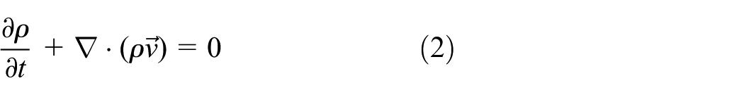
The air flow field was calculated first. The air flow field is a low-velocity viscous flow which can be calculated by Navier–Stokes (N-S) equation and solved by the Semi-Implicit Method for Pressure Linked Equations (SIMPLE) method. The N-S equation is

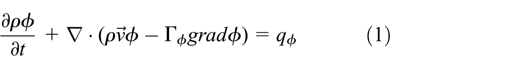
\frac{\partial ρ ϕ}{\partial t} + \nabla \cdot (ρ \vec{v} ϕ - Γ_{ϕ} grad ϕ) = q_{ϕ}

(1)

where ρ is the air density, φ is the transport variable, $\vec{v}$ is the air velocity, Γ_ϕ is the air temperature, and q_ϕ is the source item. The air has not compressed in the calculation process, so the mass conservation equation is

\frac{\partial ρ}{\partial t} + \nabla \cdot (ρ \vec{v}) = 0

(2)

The momentum equations of x, y, and z directions are

{\begin{matrix} \frac{\partial ρ u}{\partial t} + \nabla \cdot (ρ \vec{v} u - μ_{eff} grad u) = - \frac{\partial P}{\partial x} + \nabla \cdot (μ_{eff} \frac{\partial \vec{v}}{\partial x}) + ρ f_{x} \\ \frac{\partial ρ v}{\partial t} + \nabla \cdot (ρ \vec{v} v - μ_{eff} grad v) = - \frac{\partial P}{\partial y} + \nabla \cdot (μ_{eff} \frac{\partial \vec{v}}{\partial y}) + ρ f_{y} \\ \frac{\partial ρ w}{\partial t} + \nabla \cdot (ρ \vec{v} w - μ_{eff} grad w) = - \frac{\partial P}{\partial z} + \nabla \cdot (μ_{eff} \frac{\partial \vec{v}}{\partial z}) + ρ f_{z} \end{matrix}

(3)

The turbulence model used in this article is k-ε model, and the turbulent kinetic energy equation is

\frac{\partial (ρ k)}{\partial t} + \frac{\partial (ρ ε u_{i})}{\partial x_{i}} = \frac{\partial}{\partial x_{j}} [α_{k} μ_{eff} \frac{\partial ε}{\partial x_{j}}] + G_{k} + ρ ε

(4)

The turbulent energy dissipation rate equation is

\frac{\partial (ρ ε)}{\partial t} + \frac{\partial (ρ ε u_{i})}{\partial x_{i}} = \frac{\partial}{\partial x_{j}} [α_{ε} μ_{eff} \frac{\partial ε}{\partial x_{j}}] + \frac{C_{1 ε} ε}{K} G_{k} - C_{2 ε} ρ \frac{ε^{2}}{k}

(5)

It is an unsteady model. The diffusion term is solved by central-difference, and the convection term is solved by second-order upwind scheme. And

μ_{eff} = μ_{l} + μ_{t} = μ_{l} + ρ c_{μ} k^{2} / ε

(6)

G_{k} = μ_{t} (\frac{\partial u_{i}}{\partial x_{f}} + \frac{\partial u_{j}}{\partial x_{i}}) \frac{\partial u_{i}}{\partial x_{j}}

(7)

μ_{t} = C_{μ} ρ k^{2} / ε

(8)

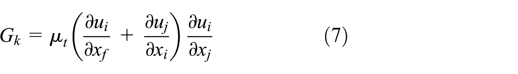
where ρ is the air density, k is the turbulent kinetic energy, ε is the turbulent dissipation rate, u_i and u_j are the air velocities, t is the turbulent time scale, α_k is the Prandtl number of k equation, α_ε is the Prandtl number of ε equation, µ_eff is the coefficient of turbulent viscosity, G_k is turbulent kinetic energy generated by the laminar velocity of gradient, and C_1ε and C_2ε are the empirical coefficients. C_1ε = 1.44, C_2ε = 1.92, C_µ = 0.09, α_k = α_ε = 1.39, σ_k = 1.0, σ_ε = 1.22, and σ_t = 0.9–1.0.

The impingement limit was calculated by the Lagrangian method and solved based on Runge–Kutta method. The initial time-step used in the trajectory integration is 10⁻⁵ s. The Lagrangian equation is shown as follows

M_{d} \frac{d^{2} {\vec{x}}_{d}}{d t^{2}} = (ρ_{d} - ρ_{a}) V_{d} \vec{g} + \frac{1}{2} C_{d} A_{d} ρ_{a} | {\vec{u}}_{a} - {\vec{u}}_{d} | ({\vec{u}}_{a} - {\vec{u}}_{d})

(9)

where ρ_d is the density of droplets, ρ_a is the density of air, $\vec{g}$ is the acceleration of gravity, A_d is the area of water droplet facing wind, V_d is the volume of water droplet, C_d is drag coefficient, ${\vec{u}}_{a}$ is the local wind velocity, and ${\vec{u}}_{d}$ is the water droplet velocity. The Runge–Kutta equation is

{\vec{u}}_{n + 1} = {\vec{u}}_{n} + \frac{1}{6} (t_{n + 1} - t_{n}) (K_{1} + 2 K_{2} + 2 K_{3} + K_{4})

(10)

where ${\vec{u}}_{n + 1}$ is the value of next time; ${\vec{u}}_{n}$ is the current value; K₁ is the slope of the beginning time; K₂ is the slope of the midpoint of the time; K₃ is also the slope of the midpoint of the time, but this value is determined by K₂; and K₄ is the slope of the end time, it is determined by K₄.

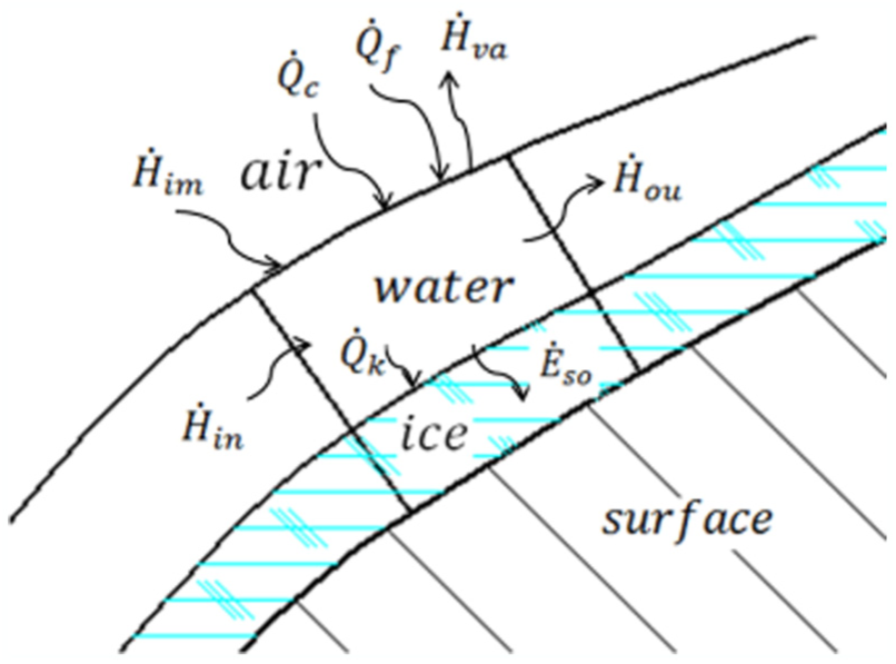
Based on the control body theory, the process of icing which droplets impact on blade is solved by mass and energy conservation equations. The principal of mass and energy conservation on the surface of single control body is shown in Figures 3 and 4.

Figure 3.

Mass conservation in single control body.

Figure 4.

Energy conservation in single control body.

According to the mass conservation, the weight of current control body equals to the difference between mass of water going into the surface of control body and the leaving ones. The equation is

m'_{in} + m'_{im} - m'_{va} - m'_{ou} = m'_{so}

(11)

Formula (11) is usually given as

m'_{ou} = (1 - f) (m'_{im} + m'_{in}) - m'_{va}

(12)

where $m'_{in}$ is mass of water flow from upstream into control body, $m'_{im}$ is the super-cooled droplets impacting on the blade, $m'_{va}$ is the mass of water transforming into steam by evaporation or sublimation, $m'_{ou}$ is the mass of water droplets which do not freeze and flow into downstream, $m'_{so}$ is the mass of water which was changed to ice, and f is the icing ratio.

The surface energy of the control body is subdivided into eight items. According to the first law of thermodynamics, the energy balance equation is

{\overset{\cdot}{E}}_{so} + {\overset{\cdot}{H}}_{va} + {\overset{\cdot}{H}}_{ou} - {\overset{\cdot}{H}}_{in} - {\overset{\cdot}{H}}_{im} = {\overset{\cdot}{Q}}_{f} - {\overset{\cdot}{Q}}_{c} - {\overset{\cdot}{Q}}_{k}

(13)

where ${\overset{\cdot}{E}}_{so}$ is the energy of water during freezing, ${\overset{\cdot}{H}}_{va}$ is the heat of evaporation of water droplets or ice surface, ${\overset{\cdot}{H}}_{ou}$ is the energy of droplets out the body, ${\overset{\cdot}{H}}_{in}$ is the energy of droplets into the body, ${\overset{\cdot}{H}}_{im}$ is the impact kinetic energy into the water heat flux, ${\overset{\cdot}{Q}}_{f}$ is the energy of air friction heating, ${\overset{\cdot}{Q}}_{c}$ is the convective hot flow of wall and the environment, and ${\overset{\cdot}{Q}}_{k}$ is the heat between ice and water.

Meshing

Figure 5 shows the main information about computational domain and meshing around the airfoil. C-type meshing was applied in this research. The standard wall functions method was used in this article. The inner node P was located in the logarithmic law layer which is the vigorous turbulent area. The y+ was set as 50 in this research. And, the semi-empirical formula u+ = 2.5ln(y+) + 2.5 was used to related the quantities on the wall with the unknown quantities in the turbulent core area which should be solved. To accurately calculate the flow field changing around the surface of airfoil, the grids around the airfoil are encrypted and represented.

Figure 5.

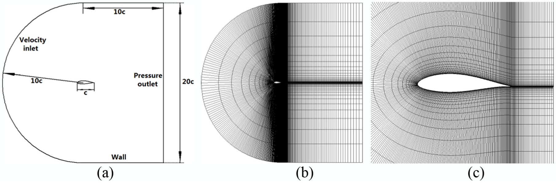
Mesh around blade airfoil: (a) simulation field, (b) meshing, and (c) meshing around airfoil.

For researching the best grid number to simulate, the grid independence verification test was carried out, and the result is shown in Figure 6. The verification was based on the lift coefficient of section 1 airfoil. The result shows that the line of lift coefficient tends to be steady when the grid numbers are more than 36,000. Therefore, the number of grid was set more than 36,000 under per simulation in this article.

Figure 6.

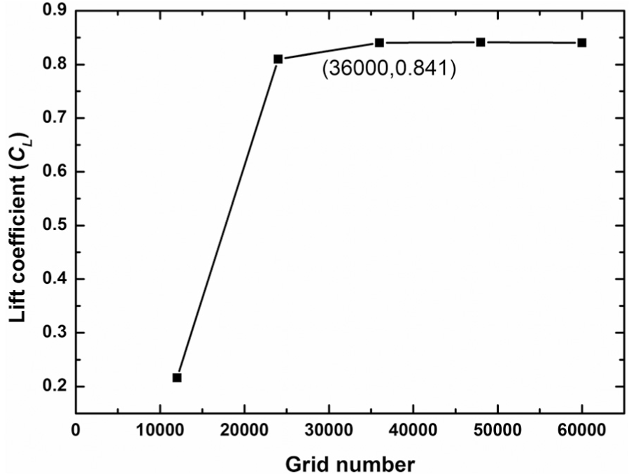
Meshing independence verification.

Table 2 shows the material properties of water and ice. Table 3 shows the main environmental parameters including temperature, liquid water content (LWC), medium volume droplet (MVD), and icing time. Eight temperature values from −6°C to −20°C were selected to invest the effects of temperature on icing under the certain LWC and MVD. Three icing times were decided to research the ice accretion on blade surface with the increase in the time.

Table 2.

Material properties of water and ice.

Material	ρ (g m⁻³)	µ (Pa s)	q (J kg⁻¹)	c (J (kg °C)⁻¹)
Water	1000	1.7921 × 10⁻³	2.48 × 10⁶	4200
Ice	800	–	3.35 × 10⁵	2100

Table 3.

Environmental parameters for simulation.

Temperature (°C)	LWC (g m⁻³)	MVD (µm)	t (s)
−6
−8
−10			1800
−12	0.5	30	3600
−14			5400
−16
−18
−20

LWC: liquid water content; MVD: medium volume droplet.

Validation

To verify the feasibility of the simulation method used in this study, a validation was carried out with past researches including simulation and icing wind tunnel tests.¹⁹ The model was decided as the NACA0012 airfoil and was in static condition at the attack angle of 0°. Two other computational codes were selected including IRC Code established by China Aerodynamics Research and Development Center and Messinger Model established by Messinger for validation. The simulation conditions are shown in Table 4. Figure 7 shows the results of icing shapes on airfoil by different methods. The icing shapes obtained by different methods have good agreement, in general, although there still exist some differences between each other. Therefore, the icing shape obtained using the method in this study can be used as qualitative analysis for evaluating the icing distribution characteristics.

Table 4.

Simulation conditions.

Condition	U _∞ (m s⁻¹)	P (Pa)	T (°C)	LWC (g m⁻³)	MVD (µm)	t (min)
No. 1	67.05	101,300	−6.1	1.0	20	6
No. 2	67.05	101,300	−28.4	1.0	20	6

LWC: liquid water content; MVD: medium volume droplet.

Figure 7.

Comparison between other codes and experiments: (a) comparison 1 and (b) comparison 2.

To verify that the Quasi-3D simulation method could be used to calculate the icing accretion on rotating blade, the icing test was carried out. Figure 8 shows the diagram of test. The NACA0018 blades were installed on the rotating beam to simulate the icing accretion on the cross section of the airfoil of the wind turbine blade. Two installed angles were set in this icing test. The test conditions are as follows: LWC = 0.5 g m⁻³, MVD = 50 µm, T = −15°C, U = 6 m s⁻¹, n =600 r min⁻¹, and t = 225 s. Figure 9 shows the comparison results between experiment and simulation. The comparison results show that the results of simulation are in agreement with the results of experiment. The result shows that this Quasi-3D simulation method could be used to calculate the icing accretion on rotating blade of wind turbine.

Figure 8.

The diagram of test.

Figure 9.

Comparison between simulations and experiments: (a) α=0°; and (b) α=10°.

Results and discussion

Icing distribution

Figure 10 shows icing shapes of sections of 2, 4, 6, and 8 under different temperatures at the icing time of 5400 s. The icing shape changes with temperature variation. It is observed that horn icing shape occurs at the temperatures between −6°C and −14°C, and streamline icing shape occurs at the temperature of −20°C. The icing shapes have the typical characteristics of both the horn shape and streamline shape when the temperature is between −16°C and −18°C. When moist air impacts on the blade, it forms water film to spread from middle to two sides due to the effect of flow wind at the temperatures between −6°C and −14°C, thereby forming concave area on the blade. This is in contrast to water film being not formed due to the effect of freezing on the blade immediately at the temperature of −20°C.

Figure 10.

Icing shapes of different sections at different temperatures and icing time of 5400 s: (a) section 2, (b) section 4, (c) section 6, and (d) section 8.

Figure 11 shows ice accretion characteristics on different blade sections at various simulated times ranging from 1800 to 5400 s. It is found that the horn icing shape occurs on different blade sections at temperature of −6°C, and ice accretion thickness increases with the passing of time at certain sections. When the temperature decreases by −20°C, icing shape changes from horn to streamline, and the streamline ice accretion thickness increases with the passing of time at certain sections.

Figure 11.

Icing shapes of different sections at different temperatures: (a) icing shapes of different airfoils at temperature of −6°C, (b) icing shapes of different airfoils at temperature of −14°C, and (c) icing shapes of different airfoils at temperature of −20°C.

The 3D icing shape on blade surface is shown in Figure 12 using quasi-3D numerical simulation reported by Li et al.²⁶ According to the quasi-3D model, closer the section to the blade tip, bigger the icing shape is. The water content increases due to the high tangential velocity close to the blade tip, thereby forming big icing shape. When icing accretes on the blade tip, the performance of wind turbine reduces due to torque variation.

Figure 12.

Quasi-3D icing shape: (a) horn icing shape and (b) streamline icing shape.

Analysis of dimensionless parameters of icing shape

The dimensionless parameters including icing area, stationary thickness, and icing volume are selected to analyze ice accretion characteristics on blade surface.²⁷

Figure 13 shows the typical characteristic parameters of streamline icing shape and horn icing shape. The typical characteristic parameters of streamline icing shape include icing area S, stationary point thicknessδ, stationary point deflect angle θ, icing upper limit L_u, icing lower limit L_d, and width of icing w. And, the typical characteristic parameters of horn icing shape including icing area S, icing upper limit L_u, icing lower limit L_d, width of icing w, upper horn δ_u, thickness of lower horn δ_d, deflection angle of upper horn θ_u, and deflection angle of lower horn θ_d.

Figure 13.

Typical characteristics of different icing shapes: (a) streamline icing shape and (b) horn icing shape.

The typical characteristic parameters including icing area, the maximum stagnation thickness, and icing volume are represented by S, δ_max, and V for evaluating the icing shapes of blades, respectively. Dimensionless parameters including the maximum stationary thickness, icing area, and volume are expressed as follows. The maximum stationary point thickness of streamline icing shape is

δ \max = δ

(14)

The maximum stationary point thickness of horn icing shape is

δ_{\max} = \max [δ, δ_{u}, δ_{d}]

(15)

η_{σ} = \frac{δ}{c}

(16)

η_{S} = \frac{S}{S_{b}}

(17)

η_{V} = \frac{V_{i}}{V_{b}}

(18)

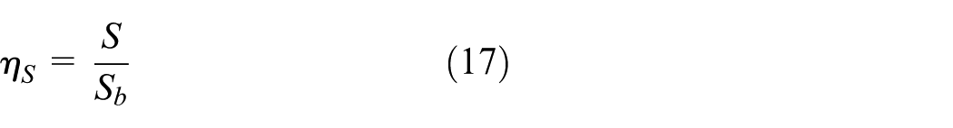
where δ is the stationary point thickness, δ_u is the upper stationary point thickness, δ_d is the dower stationary point thickness, c is the chord length of airfoil, S is the icing area, S_b is surface area of blade, V_i is the volume of icing, and V_b is the volume of blade.

Figure 14 shows the relationship between icing area and temperature on different blade sections at time of 5400 s. The icing area increases with decreasing the temperatures. The icing area rises rapidly at the temperatures between −6°C and −12°C, and the icing area rises slowly when the temperatures are between −14°C and −20°C. In addition, the effect of environmental temperature on the icing area close to the blade tip is significant. When environmental temperature is −20°C, icing area reaches 43% of airfoil area, and the maximum icing area is 2.8 × 10⁶ mm². This is mainly because the water content increases close to the blade tip due to high tangential velocity, thereby freezing immediately at temperature of −20°C.

Figure 14.

The relationship between icing area and temperatures on different blade sections at time of 5400 s.

Figure 15 shows relationship between the maximum dimensionless stationary point thickness of different sections and different temperatures at time of 5400 s. The maximum dimensionless stationary point thickness first increases with the temperatures decreasing from −6°C to −12°C, then decreases with the temperatures reducing from −12°C to −20°C. The maximum stationary thickness is 220 mm at the temperature of −12°C, which is about 29% of the airfoil chord length. This is due to the fact that horn icing shape with two horns occurs at the temperatures between −6°C and −12°C, thereby increasing the maximum stationary thickness.

Figure 15.

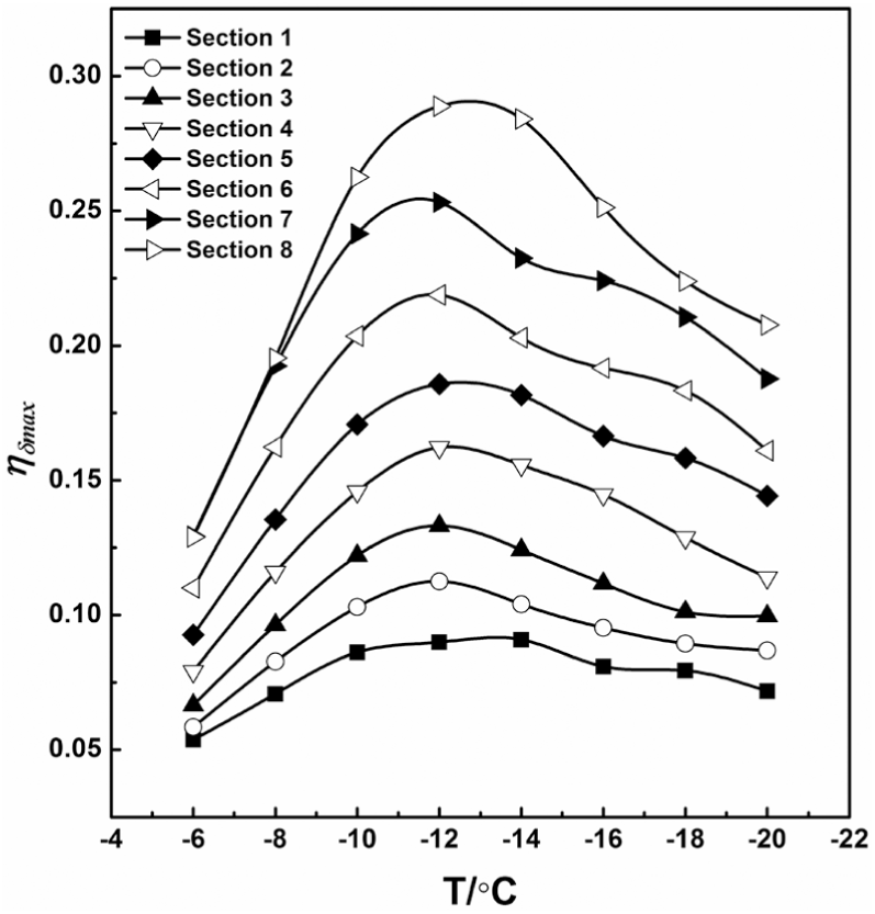
The relationship between the maximum dimensionless stationary point thickness of different sections and different temperatures at time of 5400 s.

Figure 16 shows the relationship between dimensionless icing volume of blade and different temperatures at different times. The icing volume increases with temperature decreasing generally. At the initial icing process, the icing volume of blade increases layer by layer and keeps the similar type with increasing time due to the effect of decreasing temperatures. Therefore, the maximum icing volume is 2.04 × 10⁸ mm³, which is about 14% of the blade volume.

Figure 16.

The relationship between dimensionless icing volume of blade and different temperatures at different times.

Flow field

Figure 17 shows the flow field around blade airfoil of section 8 with and without icing under different icing times. Figure 17(a) shows the change of flow field around blade airfoil with increasing icing times at −14°C, which is the horn ice shape. Figure 17(b) shows the change of flow field around blade airfoil with increasing icing times at −20°C, which is the streamline ice shape. Comparing with the airfoil without icing, the flow field around airfoil with streamline ice changed slightly near the leading edge. However, the flow field changed greatly for horn ice condition. According to Figure 17(a), the flow field almost completely changed at the position of horn icing. According to Figure 17(b), the streamline changed and the negative pressure zone appeared on the abdomen of the airfoil. The negative pressure zones appear on both sides of airfoil surface. It can be concluded that the aerodynamic characteristics of iced blade will be definitely greatly decreased, which can lead to the whole power performance degradation of wind turbine.

Figure 17.

Flow field around the airfoil at different icing times under different temperatures: (a) T = −14°C and (b) T = −20°C.

Conclusion

The main conclusions obtained under the condition of this study are as follows:

Two icing shapes are obtained for all blade sections studied at different temperatures: horn icing shape and streamline icing shape. The horn icing shape occurs at the temperatures between −6°C and −14°C and the streamline icing shape occurs at the temperature of −20°C. The icing shapes have the typical characteristics of both the horn shape and streamline shape when the temperature is between −16°C and −18°C.

At certain temperature, the icing shapes of different sections along the turbine blade are different. Closer the section to the blade tip, bigger the icing shape is.

At certain blade section, the icing accretes layer by layer on airfoil surface and keeps the similar icing shape with the increase in the time for all temperatures researched in this study.

The icing area at certain sections increases with decrease in the temperature. The maximum icing area obtained in this study reaches 43% of the airfoil area. The whole icing volume also increases with decrease in the temperature generally and the maximum icing volume is about 14% of blade volume.

Footnotes

Appendix 1

Handling Editor: MA Hariri-Ardebili

Declaration of conflicting interests

The author(s) declared no potential conflicts of interest with respect to the research, authorship, and/or publication of this article.

Funding

The author(s) disclosed receipt of the following financial support for the research, authorship, and/or publication of this article: This research was supported by the National Natural Science Foundation of China (NSFC; Nos 51576037 and 11172314) and National Key Basic Research Program of China (No. 2015CB755800). The authors thank their supports.

ORCID iD

Yan Li

References

Zhang

Tang

Niu

et al . Wind energy rejection in China: current status, reasons and perspectives. Renew Sust Energ Rev 2016; 66: 322–344.

Zhao

Qian

Zheng

et al . Enhancement approaches of aerodynamic performance of lift-type vertical axis wind turbine considering small angle of attack. J Drain Irrig Mach Eng 2018; 36: 146–153.

Zhao

Tagawa

et al . Starting performance effect of a truncated-cone-shaped wind gathering device on small-scale straight-bladed vertical axis wind turbine. Energ Convers Manage 2018; 167: 70–80.

Buckley

Watson

Cahill

et al . Mitigating the structural vibrations of wind turbines using tuned liquid column damper considering soil-structure interaction. Renew Energ 2018; 120: 322–341.

Liu

A new fault diagnosis approach for the pitch system of wind turbines. Adv Mech Eng 2017; 9: 1–9.

Zhang

Liu

Xian

et al . A review of methods for vortex identification in hydroturbines. Renew Sust Energ Rev 2018; 81: 1269–1285.

Zeng

Song

Research on experiment and numerical simulation of ultrasonic de-icing for wind turbine blades. Renew Energ 2017; 113: 706–712.

Han

Palacios

Schmitz

Scaled ice accretion experiments on a rotating wind turbine blade. J Wind Eng Ind Aerod 2012; 109: 55–67.

Ruff

GA.

Quantitative comparison of ice accretion shapes on airfoils. J Aircraft 2002; 39: 418–426.

10.

Zhu

Chen

et al . Numerical simulation of rime ice on NREL phase VI blade. J Wind Eng Ind Aerod 2018; 178: 57–68.

11.

Wang

Feng

et al . An icing wind tunnel experiment on the icing distribution of a blade airfoil rotating around a shaft. J Harbin Eng Univ 2017; 38: 545–553.

12.

Kraj

Bibeau

EL.

Phases of icing on wind turbine blades characterized by ice accumulation. Renew Energ 2010; 35: 966–972.

13.

Messinger

BL.

Equilibrium temperature of an unheated icing surface as a function of air speed. J Aeronaut Sci 1953; 20: 29–42.

14.

Barber

Wang

Jafari

et al . The impact of ice formation on wind turbine performance and aerodynamics. J Sol Energ Eng 2011; 133: 311–328.

15.

Ruff

Berkowitz

. Users manual for the NASA Lewis Ice Accretion Prediction Code (LEWICE). Technical report, NASA-CR-185129, May1990.

16.

Wright

. Users manual for the improved NASA Lewis ice accretion code LEWICE 1.6. Technical report, NASA-CR-198355, 1June1995.

17.

Potapczuk

Bidwell

CS.

Numerical simulation of ice growth on a MS-317 swept wing geometry. Technical report, AIAA-91-0263, 1January1991. Reston, VA: AIAA.

18.

Hedde

Guffond

Development of a three-dimensional icing code comparison with 3D experimental shapes. AIAA-92-0041, January1992. Reston, VA: AIAA.

19.

Xian

Numerical computation of aircraft icing and study on icing test scaling law. PhD Thesis, China Aerodynamics Research and Development Center Graduate School, Mianyang, China, 2007.

20.

Wang

K-C

H-L

et al . 3-D numerical simulation of droplet collection efficiency in large-scale wind turbine icing. Acta Aerodyn Sin 2013; 31: 745–751.

21.

Shu

Liang

et al . Study on small wind turbine icing and its performance. Cold Reg Sci Technol 2017; 134: 11–19.

22.

Shu

et al . 3D numerical simulation of aerodynamic performance of iced contaminated wind turbine rotors. Cold Reg Sci Technol 2018; 148: 50–62.

23.

Wang

Liu

et al . Characteristics of ice accretions on blade of the straight-bladed vertical axis wind turbine rotating at low tip speed ratio. Cold Reg Sci Technol 2018; 145: 1–13.

24.

Tagawa

Feng

et al . A wind tunnel experimental study of icing on wind turbine blade airfoil. Energ Convers Manage 2014; 85: 591–595.

25.

Wang

et al . An icing wind tunnel test on icing characteristics of cylinder rotating around a shaft. Acta Aeronaut Et Astronaut Sin 2017; 38: 116–126.

26.

Wang

Sun

et al . Icing distribution of rotating blade of horizontal axis wind turbine based on Quasi-3D numerical simulation. Therm Sci 2018; 22: S681–S691.

27.

Wang

Numerical simulation and icing wind tunnel test study on icing distribution on rotating blade of horizontal axis wind turbine. Harbin, China: Northeast Agricultural University, 2017.

Temperature effect on icing distribution near blade tip of large-scale horizontal-axis wind turbine by numerical simulation

Abstract

Keywords

Introduction

Geometric model and method

Wind turbine model

Numerical simulation

Meshing

Validation

Results and discussion

Icing distribution

Analysis of dimensionless parameters of icing shape

Flow field

Conclusion

Footnotes

Appendix 1

Declaration of conflicting interests

Funding

ORCID iD

References