
Abstract
An experimental and analytical method to evaluate the performance of a loop-type wind turbine generator is presented. The loop-type wind turbine is a horizontal axis wind turbine with a different shaped blade. A computational fluid dynamics analysis and experimental studies were conducted in this study to validate the performance of the computational fluid dynamics method, when compared with the experimental results obtained for a 1/15 scale model of a 3 kW wind turbine. Furthermore, the performance of a full sized wind turbine is predicted. The computational fluid dynamics analysis revealed a sufficiently large magnitude of external flow field, indicating that no factor influences the flow other than the turbine. However, the experimental results indicated that the wall surface of the wind tunnel significantly affects the flow, due to the limited cross-sectional size of the wind tunnel used in the tunnel test. The turbine power is overestimated when the blockage ratio is high; thus, the results must be corrected by defining the appropriate blockage factor (the factor that corrects the blockage ratio). The turbine performance was corrected using the Bahaj method. The simulation results showed good agreement with the experimental results. The performance of an actual 3 kW wind turbine was also predicted by computational fluid dynamics.
Keywords
Introduction
Renewable energy sources are gaining increasing interest, as they play a significant role in satisfying growing energy demands. Companies involved in the production of commercial wind power generators are already producing large megawatt (MW) class wind turbines, with rotor diameters exceeding 100 m. On the other hand, no significant attention has been paid to the production of small wind turbines until recently, when they started to attract attention due to the global investments and research in smart grid projects. Smart grids can maximize energy efficiency by integrating information and communication technologies into electric power grids, and monitoring electricity usage and supply in real time. Based on these information and communication technologies, small-sized power generation systems have emerged in the smart grid context, because prosumers produce electricity at the same time as existing users consume electricity. Wind power generators (together with solar energy sources) are used for small power generation systems, because solar cells cannot solely generate sufficient power to meet the demand. Unlike large wind power generators, small wind power systems that are connected to such self-sufficient power supply systems are typically located near residential complexes. However, installing wind turbines near to residential areas inevitably causes noise problems due to the aerodynamic low-frequency wind turbine noise, which may lead to both physical and psychological detrimental effects such as nervous breakdowns and insomnia.1,2 The main origin of this aerodynamic noise is the tip vortex that occurs at the blade tip when the blade rotates at high speed. As the loop-type wind turbines examined in this study are characterized by their ability to generate high torque at low speed, the rotational speed of the turbine is half of that of a conventional turbine, and the blade tips are closed. Therefore, much less aerodynamic noise is caused by the tip vortex of wind turbines. 3 Such turbines are structurally stable, because each two blades form one blade with small blade deformation, leading to low vibration and a long lifespan. This wind turbine capability to generate high torque at low rotation speeds can be attributed to the fact that it has optimal tip speed ratio (TSR) at low rotation speed, because of its larger solidity compared to the blade type turbine, as shown in Figure 1. TSR is defined as equation (1) as the ratio of blade tip to inflow wind velocity

where

where n is number of blades and D is wind travel distance through the turbine. And the solidity


Comparison of solidity between conventional wind turbine blade and loop-type wind turbine blade (left: conventional wind turbine blade; right: loop-type wind turbine blade).
Many parameters such as inflow angle (
As the purpose of this study is to investigate the performance of 3 kW small wind turbines, studies conducted on small wind turbines have been reviewed. Mayer et al. 11 examined the change in the initial motion pattern of a wind turbine according to the pitch angle of a small 5 kW wind turbine and found that the idling time of the wind turbine decreased as the pitch angle increased. Wright and Wood 12 discussed the torque generation and power characteristics of small wind turbines. Howell et al. 13 conducted experiments using CFD (2D and 3D) to evaluate the performance of a small vertical axis wind turbine (VAWT). Neal and Clark 14 proved that using a soft stall (electrical loading control) on a 900 W small wind turbine improves its power generation.
Even if the wind turbine is small, because the blade length exceeds 1 m it is necessary to conduct experiments in wind tunnel using a reduced scale models. Choo 15 conducted an experiment by mounting a scale model on a vehicle to analyze the aerodynamic of a wind turbine using a 1/48 scale model of a 5 MW offshore wind turbine. Zaghi et al. 16 studied the blockage effect in wind tunnel tests through simulations and experiments. Wang et al. 17 analyzed the performance of a cross-axis wind turbine (CAWT) using a wind tunnel test. The performance of the tested CAWT was compared with that of a typical VAWT. As no research has ever been conducted on evaluating the performance of loop-type wind turbines, this study is aimed to examine the performance of a miniature model of a loop-type wind turbine and predict the performance of an actual wind turbine.
A 1/15 scale model of a previously designed 3 kW loop-type wind turbine (manufactured using a 3D printer) is used in this study. The obtained results are compared to the experimental and flow analysis results, to verify the validity of the CFD analysis. Then, 3D simulations of the tested 3 kW wind turbine are performed, to predict the performance of a full sized wind turbine.
Design of loop-type wind turbine
The basic form and components of the loop-type wind turbine blade are shown in Figure 2. The blade is divided into two portions, a front end and a rear end. The spine line forms the overall blade shape, and the airfoil forms the shape of the blade along the spine line. The shape of the airfoil shown in Figure 2 is not the commonly used airfoil developed by the National Advisory Committee for Aeronautics (NACA) or National Renewable Energy Laboratory (NREL). It is an arc-shaped airfoil, similar to that used in a VAWT. The front and rear blades of the loop-type turbine have slightly different roles. The front blades can achieve high efficiency at low speeds, and the rear blades are designed to achieve high efficiency at high speeds.

Schematic of loop-type wind turbine blade.
The design of the 3 kW loop-type wind turbine tested in this study is well documented in a study by Kim et al.
18
The overall design process is shown in Figure 3. First, the diameter of the wind turbine was set by reversing Betz’s law to determine the size of the wind turbine corresponding to the power. Meanwhile, the power coefficient


Block diagram of blade design process.
where
In the abovementioned design study, qualitative comparisons of the scaled models were carried out. In this study, the previously designed A model turbine is quantitatively evaluated.
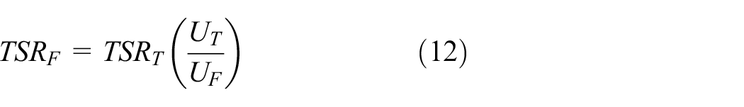
A proper similarity law should be applied for the quantitative evaluation of the tested wind turbine. As a 1/15 scale experimental model is used for the wind tunnel test, two similarity laws can be applied to the model wind turbine, Reynolds number similarity, and TSR similarity. The Reynolds number range of the miniature model is

Numerical study
FLUENT (version 18.2; ANSYS Inc., Canonsburg, PA, USA) was utilized to perform the 3D numerical analysis. The time domain is classified into two types: steady state and transient state. The spatial domain (flow field) is commonly used for steady and transient analysis. The 1/15 scale model is located at the center of the flow field when viewed from the front. The cross section of the flow field is 1500 mm × 1500 mm and the length is 2600 mm. The steady-state analysis is a simulation that changes the rotational velocity at the same constant flow rate as in the wind tunnel test (TSR controlled state). The angular velocity was controlled to 250–1000 r/min. The transient state (no-load state) analysis can confirm the movement from the stop of the turbine to the steady state. All movements except the axial rotation of the turbine were limited (1-degree-of-freedom movement). The angular velocity of the turbine is measured using transient simulations when the rotational velocity of the turbine no longer increases (i.e. in the state of aerodynamic equilibrium). This confirms the maximum rotational speed of the blade under ideal conditions. The numerical analysis allows an appropriate setting of the turbine rotation speed during the steady-state simulation.
Geometry and grid generation
The domain of analysis is shown in Figure 4. The entire area is divided into a stop area and a rotation area, and an interface is created to interpolate data between these areas. The width and height of the flow field were set to five times the radius of rotation to avoid wall effect. The length of the flow field was 10 times the radius of rotation to sufficiently simulate the wake region.

Flow fields and boundary conditions for 3D numerical simulation.
Mesh is generated using ANSYS Meshing (version 18.2; ANSYS Inc.). The elements started with a fine mesh on the blade surface to gradually form a rough mesh that expresses the complex shape of the blade. The growth rate of the mesh is set to 1.1; thus, the mesh gradually grows to avoid excessive deterioration of mesh quality. The mesh used in the analysis was approximately 3.3 million polyhedral. Because of the complexity of the curve forming the blade surface, skewness and orthogonal quality metrics were used to determine the mesh quality. The skewness was set at less than 0.75 and the orthogonal quality was more than 0.38, except for some blade surface grids. Using mesh quality metrics is considered suitable for numerical simulations due to the improved grid quality provided in FLUENT.
The blade surface utilized the inflation function to create a layer of prismatic meshes. Five layers are used with growth rate of 1.2. The height of the first grid was 0.12 mm. The value of


Solver setting
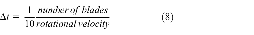
Transient analysis that employs dynamic mesh and turbine mass and moment of inertia is performed to determine the ideal maximum rotational velocity of the turbine during no-load operation. In order to appropriately perform the analysis, small time steps must be used because of the fast rotation velocity of turbine. Although this method involves time-consuming computations, it can properly express the turbine motion, which cannot be shown by a steady-state analysis using a moving reference frame (MRF). The time step is set to 0.005 s. The time step of the transient turbo machine is recommended as shown in equation (8)
Steady-state analysis using the MRF method was performed to confirm the force applied to the turbine at specific wind velocity and rotational velocity of turbine. This can be used to verify the torque and power of turbine.
Parallel computing is used to minimize the computation time. The flow field is divided into 16 compartments, which can be allocated to each core (Intel Xeon E5-2630v3 × 2) to utilize all the computer resources. A pressure-based solver was used for incompressible flow. The viscous model employed for this CFD analysis is shear stress transport (SST)
Experimental study
Wind tunnel
To test the performance of the 3 kW loop-type wind turbine without directly producing a prototype, a 1/15 scale model was used to conduct the wind tunnel experiment. A schematic diagram of the experiment is shown in Figure 5. The wind tunnel used in the experiment is an open type with a maximum wind speed of 12 m/s and a turbulence intensity of under 2.5%. It has a 1000 × 1000 mm rectangular test section. The wind is stabilized by the flow straightener installed at the inlet and then flows into the test section. The wind velocity inside the wind tunnel is monitored in real time using 16 hot-wire anemometers (UAS 1500, °C Port 3600; Degree Controls Inc., Milford, NH, USA) placed in front of the test section. If the diameter of the turbine is denoted as D, the position at which the flow velocity is measured must be 2D. When the reference wind velocity measurement position is located close to the turbine, the air flow is stagnated by the turbine and the wind speed is measured to be low. This causes the turbine power coefficient to be overestimated. If the flow velocity is measured from too far away, the wind speed will not yet be stabilized, and the correlation between the reference wind speed and the power becomes low. According to the International Electrotechnical Commission (IEC 61400) standard, the flow velocity of horizontal axis wind turbine (HAWT) should be measured from a distance 2 to 4 times the rotor diameter.
21
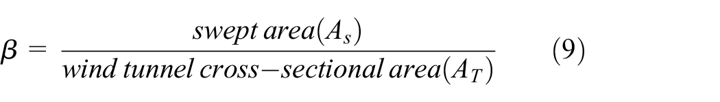
Obstacles in the wind tunnel disturb the flow in the test section. The inner wall of the wind tunnel can be regarded as an obstacle. Therefore, the cross-sectional area of the wind tunnel and the area occupied by the test subject should be considered in order to prevent any change in the flow velocity caused by the wall and test subject when the flow passes around the test subject. In wind tunnel tests, the blockage ratio (BR),

Schematic diagram of wind tunnel test.
BR must be less than 5% in a typical wind tunnel test. Chen and Liou 22 reported that no blockage effect correction is required for small HAWT experiments when the BR is less than 10%. With a wind turbine radius of 0.141 m and swept area of the reduced model of 0.063 m2, the BR is approximately 6%. However, a BR of approximately 18% is obtained when the area occupied by the support device for centering the turbine is considered. Therefore, it is necessary to calibrate the power coefficient after the experiment. 23
Small-scale model
A scale model was prepared using a 3D printer for the wind tunnel experiments. The nozzle thickness was 0.4 mm, and the layer thickness was 0.2 mm. The shape of the wind turbine curved surface can be expressed well using nylon filament. The turbine was printed in seven parts (turbine hub × 1, front blade × 3, rear blade × 3) and then assembled. The printed and computer-aided design (CAD) models are compared in Figure 6. The model was placed inside the wind tunnel as shown in Figure 5. The turbine was placed in the center of the wind tunnel section, and a photoelectric sensor (BS5-T1M; AUTONICS Inc., Busan, Republic of Korea) was installed on the rotating shaft to measure the rotational speed. The sensor resolution is 2000 Hz. The pulse can be measured every 90°. The photoelectric sensor was connected to a pulse meter (MP5Y-45; AUTONICS Inc.), which converted the pulse signal to angular velocity. A gear box was installed on the rotating shaft to operate the generator at an appropriate rotating velocity. The generator was connected to a multimeter (DT4252; HIOKI, Ueda, Nagano, Japan) to measure the power generated by the turbine.

Comparison of miniature CAD model and 3D printed model (left: CAD drawing; right: printed model).
Based on the experimental results, the power coefficient is determined by the TSR. The actual turbine flow cannot be determined by a miniature model experiment. However, the wind turbine rotational velocity and power coefficient are measured and compared to the results obtained by the CFD simulation to verify the reliability of the 3D analysis. Then, the actual turbine performance is predicted using the CFD analysis performed for the 3 kW turbine.
Results and discussion
Unloaded wind turbine analysis
The transient analysis was used to obtain the angular velocity of the blade over time, and the wind velocity ranged from 1.5 to 4 m/s. Figure 7 exhibits the computation results, including the angular velocity over time and the saturation time for each wind velocity. It can be seen that as the wind speed increases, the turbine rotational speed increases, and the saturation time decreases.

Angular velocity plotted against time (upper) and saturation time plotted against wind velocity (bottom).
The results of the above CFD analysis compared to the experimental results are shown in Figure 8. The range of angular velocity was 332–868 r/min in the CFD analysis and 231–641 r/min in the experiment. The maximum angular velocity obtained by the experiment is lower than the simulation value. This can be attributed to the loss of mechanical energy in the actual experimental apparatus. Such mechanical losses (bearing friction, loss due to vibration, etc.) were confirmed by comparing the experimental and numerical rotational kinetic energy of the turbine. The mechanical loss is defined as the difference between the rotational kinetic energy of the wind turbine through the experiment and the maximum rotational kinetic energy through CFD. The rotational kinetic energy of turbine can be expressed by equation (10), as follows
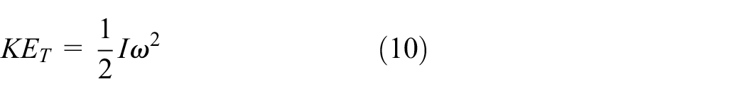
where

Maximum angular velocity plotted against wind velocity (

Kinetic energy of wind turbine and mechanical loss plotted against wind velocity (
Performance analysis
Figure 10 shows the power coefficient obtained by the wind tunnel test and CFD simulation. The CFD analysis results confirmed that the highest efficiency is achieved at

where

Power coefficient plotted against TSR (before calibration).

Comparison of expected power coefficients and calibrated experimental results.
The calibration results revealed that mostly lower power coefficient values were obtained by the experiment compared to those obtained by CFD. This is attributed to fact that the electrical power is measured in the experiment. The typical mechanical efficiency is 0.9, electrical efficiency is 0.9, and the expected power coefficient is shown during actual turbine operation. The calibrated experimental results were compared to expected power coefficient. Even though the experimental TSR of <1.1, which is much different from the expected value, the difference between the simulated and experimental TSR values is less than 10%. The power coefficient curve fit indicates that the CFD results can be considered reliable. Therefore, the performance of actual size turbines can be predicted using the simulation method applied to the small model.
Performance prediction
The CFD analysis method was used to analyze the actual scale turbine flow as the reliability of this method is confirmed as discussed above. The model was scaled up 15 times to analyze the performance of actual size turbines. Similar settings to those of the reduced scale model simulation are used. The flow velocity was fixed at 12 m/s. The results of CFD analysis are shown in Figure 12, which compares the power coefficients of the reduced scale model and the actual size turbine.

Comparison of miniature model and actual turbine performance.
When the actual turbine operates at 12 m/s, 125 r/min (λ = 2.31), it is expected power coefficient about 0.43. The power coefficient of the actual turbine is about 30% higher than that of the miniature model. The performance difference between two models is due to the Reynolds number. Low Reynolds number model shows a lower power coefficient than the actual model in the experiments.25,26 The Reynolds number affects the maximum power coefficient of the turbine because it has large effect on the lift-to-drag ratio.
Conclusion
This study aimed to evaluate the performance of a loop-type wind turbine that has never been investigated. This HAWT has a low optimal TSR to reduce aerodynamic noise. The 3 kW wind turbine is designed to deliver full power under a wind speed of 12 m/s with a TSR of 2.32. To evaluate the performance of this new turbine, a 1/15 scale 3D printed model was investigated by simultaneously using a wind tunnel test and 3D CFD analysis. The TSR similarity was applied to the reduced scale model. As the wind tunnel has a closed structure, the BR, which is the ratio of the obstacles inside the wind tunnel to the cross section, is considered. Bahaj method was employed to calibrate the BR. The CFD analysis results indicate that the point at which the reduced scale model reached the maximum power was similar to that of the optimal TSR, and the power coefficient at this point was 0.34. The experimental results revealed that the corrected power coefficient is very close to the numerical results when the electrical and mechanical losses are considered. The performance of the actual 3 kW loop-type wind turbine was predicted based on the study conducted on the reduced scale model. The power coefficient of the actual turbine was about 0.43 (when
Footnotes
Handling Editor: Ka-Veng Yuen
Declaration of conflicting interests
The author(s) declared no potential conflicts of interest with respect to the research, authorship, and/or publication of this article.
Funding
The author(s) disclosed receipt of the following financial support for the research, authorship, and/or publication of this article: This paper was supported by Kumoh National Institute of Technology.