Seismic analysis method of equipment–high rise structure–nonlinear soil system

Abstract

Based on the principle of real-time substructure shaking table test, an interactive numerical computation method which built the calculation model of each substructure in different software programs was proposed for seismic analysis of equipment–high rise structure–soil systems in order to account the effect of nonlinear soil. Considering that the response of soil under strong earthquakes does not totally enter the nonlinear stage, a locally nonlinear soil model was introduced as the numerical substructure, and the equipment–high rise structure subsystem was treated as an experimental substructure in this method. The equation of motion for the equipment–high rise structure–soil system was derived through a combination of the branch modal substructure and linear–nonlinear hybrid constraint modal substructure approaches. A 13-layer steel framework system model is used as an analytical example that the equipment–high rise structure system and local nonlinear soil computing model are built by MATLAB and ANSYS, respectively. The time histories of the system dynamic responses were obtained by interactive numerical computation, to investigate the effects of equipment–high rise structure–soil interaction on the seismic performance of the equipment and structure.

Introduction

With the rapid economic growth, large numbers of high rise structures (HRSs) have been built in the world. Besides, the proportion of equipment and other nonstructural components in buildings increases. In this context, the soil–structure interaction (SSI) becomes an increasingly important issue in seismic analysis and design of HRSs. Research revealed that the total lateral displacement of an HRS tended to increase when the behavior of soil was taken into account and that nonlinear soil properties can increase or decrease the base shear of structures compared to linear soil response, depending largely on the type of structure, seismic input frequency, and soil type.^1,2 This suggests that SSI may have an adverse effect on the structure’s response in some cases. There are many computational and experimental methods that take SSI into consideration, including finite element calculation,^3,4 on-site model excitation testing, ⁵ centrifuge testing, ⁶ and shaking table testing.^7–12 Shaking table testing, currently one of the most widely used methods, is capable of effective simulation real earthquake excitations. In this method, the shaking table platform applies seismic excitations to the structural models. To take into account SSI in shaking table tests, a soil-filled box model is usually used to represent on-site soil, and the structural system is then embedded in the ground for testing. This method requires a construction of complete test models and can be used to study the seismic responses of a structure and soil simultaneously. However, the modeling process is usually costly and technically difficult, and the size of shaking table and other limitations prevent large-scale model tests. With the development of real-time substructure testing and control techniques,^13,14 the real-time substructure shaking table test (RTSSTT) testing method has been applied to the seismic field. And the RTSSTT that includes the effect of soil^15–17 is gaining much attention. It is a huge challenge that nonlinear soil model as the numerical substructure in RTSSTT. Therefore, there is an urgent need for a more efficient and accurate computational method that considers the effect of nonlinear soil.

Considering that the response of soil under strong earthquakes does not totally enter the nonlinear stage, Wang and Jiang ¹⁸ systematically analyzed SSI using the combination of the branch modal substructure and linear–nonlinear hybrid constraint modal substructure approaches and then validated the proposed computational method by a case study. The advantages of linear–nonlinear hybrid constraint modal substructure method were also demonstrated in the dynamic analysis of three-dimensional models. ¹⁹

Based on the principle of RTSSTT, an interactive numerical computation method was proposed to achieve a simulated process of RTSSTT. This method used the linear–nonlinear hybrid constraint modal substructure approach to construct a locally nonlinear soil (LNS) model considering that the soil is not completely in nonlinear status under strong earthquakes. Then the equation of motion for an equipment–HRS–LNS system was derived using a combination of the branch modal substructure and linear–nonlinear hybrid constraint modal substructure approaches. Then this equation was transformed to obtain the equations of motion for the equipment–HRS subsystem and soil substructure for use in RTSSTT. A computational model of an equipment–HRS–soil system was selected. In this model, the HRS was a 13-story, 4-span steel frame structure, the equipment was simulated with a simplified model with a single degree of freedom (DOF), and the soil was Class III ground. The equipment–HRS subsystem was constructed using the programming software called MATLAB, and the LNS model was created using ANSYS. A comparison of the results of interactive numerical computation and integrated finite element analysis demonstrates that the analysis method proposed in this study is reliable. After that, the time histories of the equipment–HRS–soil system dynamic response were obtained by interactive numerical computation to investigate the effects of equipment–HRS–soil interaction on the seismic performance of the equipment and structure.

Derivation of the equation of motion for the equipment–HRS–LNS system

In this study, the linear–nonlinear hybrid constraint modal substructure approach was incorporated to create an LNS model, with an attempt to overcome problems such as redundancy of DOFs of soil.

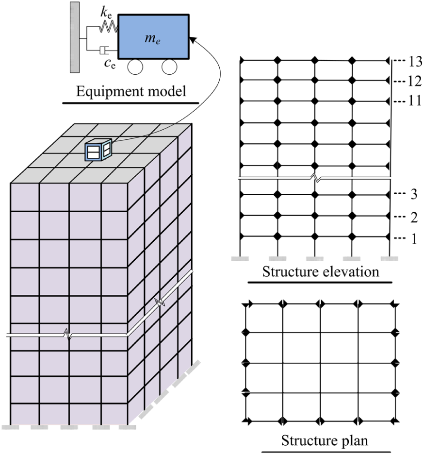
The equipment–HRS–soil system shown in Figure 1 consists of equipment, HRS, and a soil. Branch modal substructure method can be employed to derive the equation of motion for the equipment–HRS–nonlinear soil substructure β system, from which the coupling terms between the equipment–HRS subsystem and nonlinear soil substructure β can be obtained. And the equipment–HRS–nonlinear soil substructure β system was divided into branch d (equipment–HRS rigid system on nonlinear soil substructure β), which is shown in Figure 1(b), and branch s (equipment–HRS deformed system on rigid nonlinear soil substructure β), which is shown in Figure 1(c). Unlike common branch modal substructure approaches, the computational matrices for the equipment–HRS subsystem and nonlinear soil substructure β were totally preserved in this study to consider their nonlinearity separately. Later, the number of DOFs of the linear soil substructure α was reduced through the constraint modal substructure method. After coordinate transformations based on the deformation compatibility at the interface between the linear soil substructure α and nonlinear soil substructure β, the equation of motion was derived for the equipment–HRS–LNS system. The derivation process is detailed below.

Figure 1.

Derivation of the equation of motion for the equipment–HRS–LNS system. (a) Equipment–HRS–soil system. (b) Equipment–HRS rigid system on nonlinear soil substructure β. (c) Equipment–HRS deformed system on rigid nonlinear soil substructure β. (d) Reduce DOFs of linear substructure α.

As the nonlinearity of both the equipment–HRS subsystem and nonlinear soil substructure β during a strong earthquake must be considered, the computational matrices for them were preserved. The equipment–HRS subsystem displacement, u_s, can be divided into two components: the rigid body displacement caused by the motion of the nonlinear soil substructure β (Figure 1(b)) and displacement due to the motion of the subsystem itself, q_s (Figure 1(c)). u_s is calculated using equation (1)

$$\left\{u_s\right\}=\left[R\right]\left\{q_{\beta }\right\}+\left\{q_s\right\}$$

(1)

R in the equation can be determined from the equipment–HRS subsystem’s rigid body displacement produced by the deformation of nonlinear soil substructure β. The equation governing the relationship between the displacements of the equipment–HRS subsystem and nonlinear soil substructure β can be described in matrix form given by equation (2)

$$\left\{\begin{array}{c}{u}_s\hfill \\ \multicolumn{1}{c}{u_{\beta }}\end{array}\right\}=\left[\begin{array}{cc}I\hfill & R\hfill \\ \multicolumn{1}{c}{0}& I\hfill \end{array}\right]\left\{\begin{array}{c}{q}_s\hfill \\ \multicolumn{1}{c}{q_{\beta }}\end{array}\right\}$$

(2)

According to the principle of inertia coupling in a branch modal substructure method, rearranging the equation above gives the equation of motion for the equipment–HRS–nonlinear soil substructure β system (equation (3)). In the resultant equation, only the mass matrix contains coupling terms, while the stiffness and damping matrices are decoupled

$$\begin{array}{c}\left[\begin{array}{cc}{m}_s\hfill & m_{s}R\hfill \\ \multicolumn{1}{c}{R^T{m}_s}& m_{\beta }\hfill \end{array}\right]\left\{\begin{array}{c}{\stackrel{··}{q}}_s\hfill \\ \multicolumn{1}{c}{{\stackrel{··}{q}}_{\beta }}\end{array}\right\}+\left[\begin{array}{cc}{c}_s\hfill & 0\hfill \\ \multicolumn{1}{c}{0}& c_{\beta }\hfill \end{array}\right]\left\{\begin{array}{c}{\stackrel{·}{q}}_s\hfill \\ \multicolumn{1}{c}{{\stackrel{·}{q}}_{\beta }}\end{array}\right\}\hfill \\ +\left[\begin{array}{cc}{k}_s\hfill & 0\hfill \\ \multicolumn{1}{c}{0}& k_{\beta }\hfill \end{array}\right]\left\{\begin{array}{c}{q}_s\hfill \\ \multicolumn{1}{c}{q_{\beta }}\end{array}\right\}=\left\{\begin{array}{c}{f}_s\hfill \\ \multicolumn{1}{c}{f_{\beta }}\end{array}\right\}\hfill \end{array}$$

(3)

where m_s, c_s, k_s, and f_s represent the mass matrix, damping matrix, stiffness matrix, and load matrix, respectively, for the equipment–HRS subsystem in branch s; m_β, c_β, k_β, and f_β denote the mass, damping, stiffness, and load matrices, respectively, for the nonlinear soil substructure β in branch d. The computational matrices for the nonlinear soil substructure β were then repartitioned based on the types of internal DOFs i and boundary DOFs b, yielding a new equation of motion (equation (4)). In the resultant equation, $q_{\beta }^i$ and $q_{\beta }^b$ are the displacements along the internal DOFs and boundary DOFs, respectively, of the nonlinear soil substructure β

$$\begin{array}{c}\left[\begin{array}{ccc}{m}_s\hfill & m_s{R}^i\hfill & m_s{R}^b\hfill \\ \multicolumn{1}{c}{R^{\mathrm{iT}}{m}_s}& m_{\beta }^{\mathrm{ii}}\hfill & m_{\beta }^{\mathrm{ib}}\hfill \\ \multicolumn{1}{c}{R^{\mathrm{bT}}{m}_s}& m_{\beta }^{\mathrm{bi}}\hfill & m_{\beta }^{\mathrm{bb}}\hfill \end{array}\right]\left\{\begin{array}{c}{\stackrel{··}{q}}_s\hfill \\ \multicolumn{1}{c}{{\stackrel{··}{q}}_{\beta }^i}\\ \multicolumn{1}{c}{{\stackrel{··}{q}}_{\beta }^b}\end{array}\right\}\hfill \\ +\left[\begin{array}{ccc}{c}_s\hfill & 0\hfill & 0\hfill \\ \multicolumn{1}{c}{0}& c_{\beta }^{\mathrm{ii}}\hfill & c_{\beta }^{\mathrm{ib}}\hfill \\ \multicolumn{1}{c}{0}& c_{\beta }^{\mathrm{bi}}\hfill & c_{\beta }^{\mathrm{bb}}\hfill \end{array}\right]\left\{\begin{array}{c}{\stackrel{·}{q}}_s\hfill \\ \multicolumn{1}{c}{{\stackrel{·}{q}}_{\beta }^i}\\ \multicolumn{1}{c}{{\stackrel{·}{q}}_{\beta }^b}\end{array}\right\}\hfill \\ +\left[\begin{array}{ccc}{k}_s\hfill & 0\hfill & 0\hfill \\ \multicolumn{1}{c}{0}& k_{\beta }^{\mathrm{ii}}\hfill & k_{\beta }^{\mathrm{ib}}\hfill \\ \multicolumn{1}{c}{0}& k_{\beta }^{\mathrm{bi}}\hfill & k_{\beta }^{\mathrm{bb}}\hfill \end{array}\right]\left\{\begin{array}{c}{q}_s\hfill \\ \multicolumn{1}{c}{q_{\beta }^i}\\ \multicolumn{1}{c}{q_{\beta }^b}\end{array}\right\}=\left\{\begin{array}{c}{f}_s\hfill \\ \multicolumn{1}{c}{f_{\beta }^i}\\ \multicolumn{1}{c}{f_{\beta }^b}\end{array}\right\}\hfill \end{array}$$

(4)

The computational matrices for linear soil substructure α were also rearranged based on the types of internal DOFs i and boundary DOFs b. After that, the modal reduction was performed through the constraint substructure method. The corresponding coordinate transformation matrix T is given by equation (5), which consists of the dominant mode ${\varphi }_{\alpha }^N$ , constraint mode ${\phi }_{\alpha }^C$ , as well as unit vectors and null vectors

$$\left\{q_{\alpha }\right\}=\left\{\begin{array}{c}{q}_{\alpha }^i\hfill \\ \multicolumn{1}{c}{q_{\alpha }^b}\end{array}\right\}=\left[T\right]\left\{{\tilde{q}}_{\alpha }\right\}=\left[\begin{array}{cc}{\varphi }_{\alpha }^N\hfill & {\phi }_{\alpha }^C\hfill \\ \multicolumn{1}{c}{0}& I\hfill \end{array}\right]\left\{\begin{array}{c}{\tilde{q}}_{\alpha }^N\hfill \\ \multicolumn{1}{c}{{\tilde{q}}_{\alpha }^b}\end{array}\right\}$$

(5)

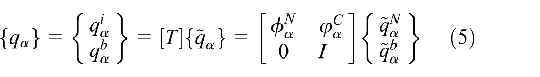
After the coordinate transformation based on the constraint modal substructure method, the equation of motion for the linear soil substructure α has the following form (equation (6))

$$\begin{array}{c}\left[\begin{array}{cc}{\tilde{m}}_{\alpha }^{\mathrm{ii}}\hfill & {\tilde{m}}_{\alpha }^{\mathrm{ib}}\hfill \\ \multicolumn{1}{c}{{\tilde{m}}_{\alpha }^{\mathrm{bi}}}& {\tilde{m}}_{\alpha }^{\mathrm{bb}}\hfill \end{array}\right]\left\{\begin{array}{c}{\stackrel{··}{\tilde{q}}}_{\alpha }^N\hfill \\ \multicolumn{1}{c}{{\stackrel{··}{\tilde{q}}}_{\alpha }^b}\end{array}\right\}+\left[\begin{array}{cc}{\tilde{c}}_{\alpha }^{\mathrm{ii}}\hfill & {\tilde{c}}_{\alpha }^{\mathrm{ib}}\hfill \\ \multicolumn{1}{c}{{\tilde{c}}_{\alpha }^{\mathrm{bi}}}& {\tilde{c}}_{\alpha }^{\mathrm{bb}}\hfill \end{array}\right]\left\{\begin{array}{c}{\stackrel{·}{\stackrel{~}{q}}}_{\alpha }^N\hfill \\ \multicolumn{1}{c}{{\stackrel{·}{\stackrel{~}{q}}}_{\alpha }^b}\end{array}\right\}\hfill \\ +\left[\begin{array}{cc}{\tilde{k}}_{\alpha }^{\mathrm{ii}}\hfill & {\tilde{k}}_{\alpha }^{\mathrm{ib}}\hfill \\ \multicolumn{1}{c}{{\tilde{k}}_{\alpha }^{\mathrm{bi}}}& {\tilde{k}}_{\alpha }^{\mathrm{bb}}\hfill \end{array}\right]\left\{\begin{array}{c}{\tilde{q}}_{\alpha }^N\hfill \\ \multicolumn{1}{c}{{\tilde{q}}_{\alpha }^b}\end{array}\right\}=\left\{\begin{array}{c}{\tilde{f}}_{\alpha }^N\hfill \\ \multicolumn{1}{c}{{\tilde{f}}_{\alpha }^b}\end{array}\right\}\hfill \end{array}$$

(6)

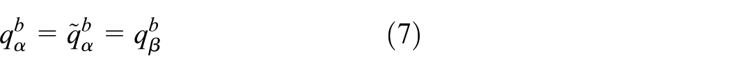
The interface between the nonlinear soil substructure β and linear soil substructure α must satisfy the following compatibility condition (equation (7))

$$q_{\alpha }^b={\tilde{q}}_{\alpha }^b=q_{\beta }^b$$

(7)

The equation of motion for the equipment–HRS–soil system was finally derived by combining the equations of motion for the linear and nonlinear soil substructures based on the condition for displacement compatibility. It is given by equation (8)

$$\begin{array}{c}\left[\begin{array}{cccc}{m}_s\hfill & m_s{R}^i\hfill & m_s{R}^b\hfill & 0\hfill \\ \multicolumn{1}{c}{R^{\mathrm{iT}}{m}_s}& m_{\beta }^{\mathrm{ii}}\hfill & m_{\beta }^{\mathrm{ib}}\hfill & 0\hfill \\ \multicolumn{1}{c}{R^{\mathrm{bT}}{m}_s}& m_{\beta }^{\mathrm{bi}}\hfill & m_{\beta }^{\mathrm{bb}}+{\tilde{m}}_{\alpha }^{\mathrm{bb}}\hfill & {\tilde{m}}_{\alpha }^{\mathrm{bi}}\hfill \\ \multicolumn{1}{c}{0}& 0\hfill & {\tilde{m}}_{\alpha }^{\mathrm{ib}}\hfill & {\tilde{m}}_{\alpha }^{\mathrm{ii}}\hfill \end{array}\right]\hfill \\ \left\{\begin{array}{c}{\stackrel{··}{q}}_s\hfill \\ \multicolumn{1}{c}{{\stackrel{··}{q}}_{\beta }^i}\\ \multicolumn{1}{c}{{\stackrel{··}{q}}_{\beta }^b}\\ \multicolumn{1}{c}{{\stackrel{··}{\tilde{q}}}_{\alpha }^N}\end{array}\right\}+\left[\begin{array}{cccc}{c}_s\hfill & 0\hfill & 0\hfill & 0\hfill \\ \multicolumn{1}{c}{0}& c_{\beta }^{\mathrm{ii}}\hfill & c_{\beta }^{\mathrm{ib}}\hfill & 0\hfill \\ \multicolumn{1}{c}{0}& c_{\beta }^{\mathrm{bi}}\hfill & c_{\beta }^{\mathrm{bb}}+{\tilde{c}}_{\alpha }^{\mathrm{bb}}\hfill & {\tilde{c}}_{\alpha }^{\mathrm{bi}}\hfill \\ \multicolumn{1}{c}{0}& 0\hfill & {\tilde{c}}_{\alpha }^{\mathrm{ib}}\hfill & {\tilde{c}}_{\alpha }^{\mathrm{ii}}\hfill \end{array}\right]\hfill \\ \left\{\begin{array}{c}{\stackrel{·}{q}}_s\hfill \\ \multicolumn{1}{c}{{\stackrel{·}{q}}_{\beta }^i}\\ \multicolumn{1}{c}{{\stackrel{·}{q}}_{\beta }^b}\\ \multicolumn{1}{c}{{\stackrel{·}{\stackrel{~}{q}}}_{\alpha }^N}\end{array}\right\}+\left[\begin{array}{cccc}{k}_s\hfill & 0\hfill & 0\hfill & 0\hfill \\ \multicolumn{1}{c}{0}& k_{\beta }^{\mathrm{ii}}\hfill & k_{\beta }^{\mathrm{ib}}\hfill & 0\hfill \\ \multicolumn{1}{c}{0}& k_{\beta }^{\mathrm{bi}}\hfill & k_{\beta }^{\mathrm{bb}}+{\tilde{k}}_{\alpha }^{\mathrm{bb}}\hfill & {\tilde{k}}_{\alpha }^{\mathrm{bi}}\hfill \\ \multicolumn{1}{c}{0}& 0\hfill & {\tilde{k}}_{\alpha }^{\mathrm{ib}}\hfill & {\tilde{k}}_{\alpha }^{\mathrm{ii}}\hfill \end{array}\right]\hfill \\ \left\{\begin{array}{c}{q}_s\hfill \\ \multicolumn{1}{c}{q_{\beta }^i}\\ \multicolumn{1}{c}{q_{\beta }^b}\\ \multicolumn{1}{c}{{\tilde{q}}_{\alpha }^N}\end{array}\right\}=\left\{\begin{array}{c}{f}_s\hfill \\ \multicolumn{1}{c}{f_{\beta }^i}\\ \multicolumn{1}{c}{f_{\beta }^b+{\tilde{f}}_{\alpha }^b}\\ \multicolumn{1}{c}{{\tilde{f}}_{\alpha }^N}\end{array}\right\}\hfill \end{array}$$

(8)

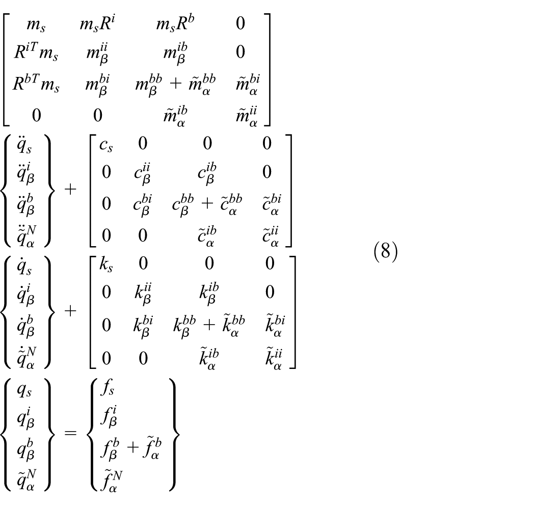
where m_sRⁱ and m_sR^b are two coupling terms in the mass matrix, representing connections between the equipment–HRS subsystem and LNS. To enable substructure testing, loads associated with the coupling terms were moved to the right-hand side of the equation, giving the equations of motion for the equipment–HRS subsystem and the LNS (equations (9) and (10))

$$m_s{\stackrel{··}{q}}_s+c_s{\stackrel{·}{q}}_s+k_s{q}_s=f_s-m_s{R}^i{\stackrel{··}{q}}_{\beta }^i-m_s{R}^b{\stackrel{··}{q}}_{\beta }^b$$

(9)

$$\begin{array}{c}\left[\begin{array}{ccc}{m}_{\beta }^{\mathrm{ii}}\hfill & m_{\beta }^{\mathrm{ib}}\hfill & 0\hfill \\ \multicolumn{1}{c}{m_{\beta }^{\mathrm{bi}}}& m_{\beta }^{\mathrm{bb}}+{\tilde{m}}_{\alpha }^{\mathrm{bb}}\hfill & {\tilde{m}}_{\alpha }^{\mathrm{bi}}\hfill \\ \multicolumn{1}{c}{0}& {\tilde{m}}_{\alpha }^{\mathrm{ib}}\hfill & {\tilde{m}}_{\alpha }^{\mathrm{ii}}\hfill \end{array}\right]\left\{\begin{array}{c}{\stackrel{··}{q}}_{\beta }^i\hfill \\ \multicolumn{1}{c}{{\stackrel{··}{q}}_{\beta }^b}\\ \multicolumn{1}{c}{{\stackrel{··}{\tilde{q}}}_{\alpha }^N}\end{array}\right\}\hfill \\ +\left[\begin{array}{ccc}{c}_{\beta }^{\mathrm{ii}}\hfill & c_{\beta }^{\mathrm{ib}}\hfill & 0\hfill \\ \multicolumn{1}{c}{c_{\beta }^{\mathrm{bi}}}& c_{\beta }^{\mathrm{bb}}+{\tilde{c}}_{\alpha }^{\mathrm{bb}}\hfill & {\tilde{c}}_{\alpha }^{\mathrm{bi}}\hfill \\ \multicolumn{1}{c}{0}& {\tilde{c}}_{\alpha }^{\mathrm{ib}}\hfill & {\tilde{c}}_{\alpha }^{\mathrm{ii}}\hfill \end{array}\right]\left\{\begin{array}{c}{\stackrel{·}{q}}_{\beta }^i\hfill \\ \multicolumn{1}{c}{{\stackrel{·}{q}}_{\beta }^b}\\ \multicolumn{1}{c}{{\stackrel{·}{\stackrel{~}{q}}}_{\alpha }^N}\end{array}\right\}\hfill \\ +\left[\begin{array}{ccc}{k}_{\beta }^{\mathrm{ii}}\hfill & k_{\beta }^{\mathrm{ib}}\hfill & 0\hfill \\ \multicolumn{1}{c}{k_{\beta }^{\mathrm{bi}}}& k_{\beta }^{\mathrm{bb}}+{\tilde{k}}_{\alpha }^{\mathrm{bb}}\hfill & {\tilde{k}}_{\alpha }^{\mathrm{bi}}\hfill \\ \multicolumn{1}{c}{0}& {\tilde{k}}_{\alpha }^{\mathrm{ib}}\hfill & {\tilde{k}}_{\alpha }^{\mathrm{ii}}\hfill \end{array}\right]\left\{\begin{array}{c}{q}_{\beta }^i\hfill \\ \multicolumn{1}{c}{q_{\beta }^b}\\ \multicolumn{1}{c}{{\tilde{q}}_{\alpha }^N}\end{array}\right\}\hfill \\ =\left\{\begin{array}{c}{f}_{\beta }^i-R^{\mathrm{iT}}{m}_s{\stackrel{··}{q}}_s\hfill \\ \multicolumn{1}{c}{f_{\beta }^b+{\tilde{f}}_{\alpha }^b-R^{\mathrm{bT}}{m}_s{\stackrel{··}{q}}_s}\\ \multicolumn{1}{c}{{\tilde{f}}_{\alpha }^N}\end{array}\right\}\hfill \end{array}$$

(10)

Then the interactive numerical computation process for the equipment–HRS–soil system was inferred from the obtained equations of motion. It involves the following steps: (1) assume that the external load and the loads associated with the coupling terms acting on the LNS at the ith step are known; (2) calculate the soil’s acceleration response at (i + Δt)th step; (3) calculate the external load and the loads associated with the coupling terms to be applied to the equipment–HRS subsystem at this step and then transmit them to it; (3) obtain the acceleration response of the equipment–HRS subsystem and the force on the LNS produced by the seismic excitation and then transmit the force to the soil for the next numerical computation. In this way, data communication between the equipment–HRS subsystem and LNS can be achieved at every step and continue until the process ends.

And the equipment–HRS subsystem model and LNS model could be created using MATLAB and ANSYS, respectively, and then they participated in the interactive numerical computation described above.

Since every step of the computational process involves data transmission, it is necessary to create a text document in each simulation software working directory to store the data transmitted. This can help the simulation software easily read the computational data during the whole computational process. For example, MATLAB uses the command loop to continuously read data in its text document, where the first line of numbers will tell whether the transmission of the computational data required is completed. If the first number is “0,” ANSYS is still computing, and thus MATLAB will continue waiting and reading the text document until the number in the first line becomes “1,” which indicates that ANSYS completed computation. After reading the data, MATLAB starts computation. The text document in ANSYS working directory works on a similar principle.

Case study

A case study of a 13-story, 4-span equipment–HRS–soil system was performed. In this system, the structure was a 13-story, 4-span steel framed building, and the equipment, a communication device placed on the floor of the top story, was simulated with a single DOF model. The soil was Class III ground.

Figure 2.

Acceleration time history curves of ground motions.

Three ground motions that are suitable for Class III ground, including El Centro, TianJin, and PerSon ground motions, were used as the seismic inputs (Figure 2). Table 2 shows the acceleration time history curves of ground motions. Then time histories of the system’s dynamic responses to the ground motions of level VIII intensity during the minor earthquake, moderate earthquake, and major earthquake stages were calculated with the acceleration amplitude adjusted to 0.7, 2.0, and 4.0 m/s², respectively. The equipment–HRS subsystem model was constructed by MATLAB programming, and the LNS model was created with ANSYS through the linear–nonlinear hybrid constraint modal substructure approach. Then both models were used in interactive numerical computations.

Equipment–HRS subsystem model

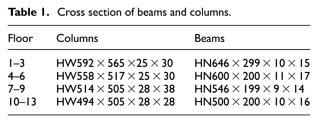
The computational model of the equipment–HRS subsystem is shown in Figure 3. The structure model was constructed of H-beam, and the cross section of each beam or column is shown in Table 1. Each story of the structure was 3.56 m high, longitudinal and transverse spans were 7.32 m. The total mass of each story was 5.86 × 10⁵ kg, except for the 13th story which weighed 5.32 × 10⁵ kg. All the beams and columns had an elastic modulus of 2.01 × 10¹¹ Pa. The yield strengths of each column and beam were 345 and 245 MPa, respectively. The damping ratio of the structure was 0.02. The equipment was simulated with a single DOF model and placed on the floor of the 13th story, and its mass was 10% of the story’s mass. Its damping ratio was 0.02 and the stiffness was 3.88 × 10⁵ N/m. The material models for the equipment and structure were both bilinear kinematic hardening models, and their post-yield stiffness were 1% of the initial stiffness values.

Figure 3.

The computational model of the equipment–HRS subsystem.

Table 1.

Cross section of beams and columns.

Floor	Columns	Beams
1–3	HW592 × 565 ×25 × 30	HN646 × 299 × 10 × 15
4–6	HW558 × 517 × 25 × 30	HN600 × 200 × 11 × 17
7–9	HW514 × 505 × 28 × 38	HN546 × 199 × 9 × 14
10–13	HW494 × 505 × 28 × 28	HN500 × 200 × 10 × 16

Based on the given parameters, a finite element model was constructed for the equipment–HRS subsystem by MATLAB programming. The beams and columns in the HRS were modeled with Euler–Bernoulli beam elements. Each beam element has two nodes, and each node has six DOFs, which are denoted u_x, u_y, u_z, u_rotx, u_roty, and u_rotz, respectively. For the structure, the mass matrix was created using the lumped mass method, and the damping matrix was based on Rayleigh damping. The single DOF equipment model was constructed of a spring-damper element. The equipment and structure were connected into an equipment–HRS subsystem model based on the displacement compatibility condition.

LNS model

Given that the soil is not totally nonlinear during strong earthquakes, an LNS model was created using the linear–nonlinear hybrid constraint modal substructure approach. The material parameters of the soil model are provided in Table 2. The LNS model has overall dimensions of 200 m × 200 m × 60 m, and a 2.50-m-thick foundation with a 31.5 m × 31.5 m cross section embedded in it.

Table 2.

Material parameters of the soil and foundation model.

Type	Depth (m)	Elastic modulus (Pa)	Density (kg/m3)	Viscous force (Pa)	Friction angle (°)
Foundation	2.5	3.12 × 1010	2570	–	–
Soil layer 1	15.0	2.43 × 107	1630	1.37 × 104	15.3
Soil layer 2	33.0	5.64 × 107	1820	1.95 × 104	16.8
Soil layer 3	12.0	3.82 × 108	2030	2.84 × 104	21.6

The modeling of the soil and mesh discretization of the LNS model was done using ANSYS. The finite element model of the soil is made up of SOLID45, an 8-node hexahedral solid element, and each node has three translational DOFs, that is, translation along the x-axis, y-axis, and z-axis, respectively. Later, the constraint equations of a rigid foundation were defined with O representing the center of the foundation and S is an arbitrary point on the foundation excepting O. Since point O is a solid element node, it has no rotational DOFs. So, the Mass21 element was introduced to this point, and the real constants were set to the smaller values. Then point O has both translational and rotational DOFs, including translation along and rotation about the x-axis, y-axis, and z-axis. The DOFs of point O and S satisfy the following relations: $u_O^x=u_S^x$ and $u_O^{\mathrm{roty}}=u_S^z/x_S$ , where $u_O^x$ and $u_S^x$ denote the displacements along the x-axis of O and S, respectively; $u_O^{\mathrm{roty}}$ denotes the angle of rotation of O about the y-axis; $u_S^z$ is the displacement of S in the z-axis direction; and x_s represents the x-coordinate of S. The LNS model was designed with a fixed bottom boundary and viscoelastic side boundaries, and the viscoelastic boundaries were simulated with Combin14, a spring-damper element provided in ANSYS.

The range of nonlinear soil will be changed under earthquakes. In order to solve the problem, Wang and Jiang ¹⁹ implemented detailed study of the range of nonlinear soil and found that the nonlinear soil scope kept within three times the size of the foundation. This conclusion was also confirmed by trial calculation. So the nonlinear soil substructure β was designed to be three times the size of the foundation which retained 11,925 DOFs, and linear soil substructure α occupied the rest of the soil model, as illustrated in Figure 4. The DOFs of the linear soil substructure α were reduced through the constraint modal substructure approach, and its 2000-order dominant mode was retained based on the principle of potential energy truncation. ²⁰ Besides, the nonlinear soil material model satisfied the Druck–Prager yield criterion. So an LNS model was created using the linear–nonlinear hybrid constraint modal substructure approach using ANSYS.

Figure 4.

Substructure division of the soil model.

Then the equipment–HRS subsystem and LNS models were used for interactive numerical computation simulating the RTSSTT of the equipment–HRS–soil system. The three ground motions mentioned above were separately inputted as required by minor, moderate, and major earthquakes with level VIII intensity to obtain seismic responses of the system.

Feasibility assessment

The results of interactive numerical computation were compared with those of the integrated finite element analysis for the purpose of assessing the feasibility of the testing method proposed in this study. In the integrated finite element analysis, an integrated model of the system was created using ANSYS. The assessment focused on the acceleration responses at the center of soil during the minor earthquake, moderate earthquake, and major earthquake stages under TianJin ground motion of level VIII intensity. Figure 5 compares the acceleration responses at the center of soil output by the two methods. During the minor earthquake, moderate earthquake, and major earthquake stages, the peak acceleration at the center of soil in the interactive numerical computation increased 4.3%, 5.5%, and 7.8%, respectively, compared with those in the integrated finite element analysis. Besides, the time histories of acceleration obtained by the two methods are generally consistent during a minor earthquake and moderate earthquake, while they differ slightly during a major earthquake.

Figure 5.

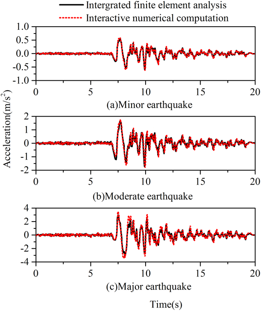
Comparison of acceleration responses at the center of soil in different computational methods.

The errors during a minor earthquake and moderate earthquake were small primarily because the soil response was linear or it experienced plastic deformation in a very limited zone in these two stages. The LNS model constructed using the linear–nonlinear hybrid constraint modal substructure approach proves to be able to capture the inherent dynamic behavior of the soil. During the major earthquake, the soil underwent relatively significant plastic deformation, and the LNS model could affect the actual seismic response of nonlinear soil behavior. Overall, the computational method incorporating the LNS model can offer the desired accuracy.

Computational efficiency is another important criterion used to assess the computational model. In this study, the number of DOFs of each model and the computation time were extracted for the two methods considered. Table 3 presents the number of DOFs of the models in the two methods. The system model created in the interactive numerical computation has 15,876 DOFs in total, a 72.5% decrease from the integrated finite element model’s DOFs 57,821. This suggests that the method proposed in this study can substantially reduce the amount of computation. Table 4 summarizes the computation time spent by each model during different earthquake stages under TianJin ground motion. MATLAB and ANSYS used the method “tic/toc” and “*get, B, active, 0, time, cpu,” respectively, to extract the computation time.

Table 3.

Number of DOFs of the models in the two computational methods.

Methods	Interactive numerical computation		Integrated finite element analysis
	MATLAB	ANSYS	ANSYS
DOFs	1951	13925	57821

DOFs: degrees of freedom.

Table 4.

Computation time for different earthquake stages in the two computational methods.

Earthquake stages	Interactive numerical computation		Integrated finite element analysis
	MATLAB (s)	ANSYS (s)	ANSYS (s)
Minor	125.62	1918.52	5873.97
Moderate	151.79	2104.92	6922.41
Major	162.01	2275.30	8262.07

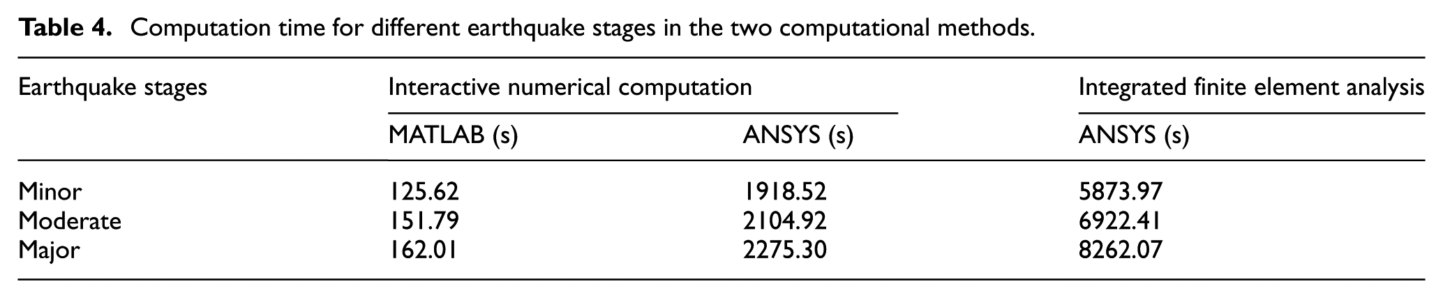
As can be seen in Table 4, the computation time spent by each software product significantly increased from minor earthquake to major earthquake in both the interactive numerical computation and integrated finite element analysis primarily because iterative computation needed to be performed after the equipment–HRS subsystem and the soil reached the nonlinear state. Besides, the total computation time spent in the interactive numerical computation method is significantly shorter than that in the other method. The computation time for the minor earthquake, moderate earthquake, and major earthquake stages were only 34.8%, 32.6%, and 29.5% of the corresponding computation time in the integrated finite element analysis. As the earthquake intensity increased, the decrease in computation time gradually accelerated. This is mainly because the LNS model used in interactive numerical computation has only a smaller number of vibration modes involved in the computation and thus avoids redundancy of DOFs. This method can significantly enhance the computational efficiency and lower the cost of computation by reducing the number of equations required for the computation and the number of iterations required to solve the nonlinear equations. Therefore, it can be employed to solve dynamic models of nonlinear systems efficiently and accurately.

Overall, the use of the LNS model can significantly improve the computational efficiency while ensuring accuracy. This confirms that the application of LNS model can provide powerful technical support for nonlinear soil participating in analysis. Meanwhile, as individual models are constructed for all substructures during interactive numerical computation, the difficulty of establishing integrated analysis model is considerably reduced. Moreover, the linear–nonlinear hybrid constraint modal substructure approach enables efficient and accurate modeling the nonlinearity of soil. The interactive numerical computation method proposed also offers an effective channel to compute and analyze complex equipment–HRS–soil systems.

The advantage of the proposed method lies in that the use of the LNS model can significantly improve the computational efficiency while ensuring accuracy. And interactive numerical computation can reduce the difficulty of modeling. However, the shortcoming of the proposed method lies in that it may be hard for the engineers for its demands of program skills and expertise.

Computation and analysis

To analyze the impact of equipment frequency changes in different systems, an equipment–HRS subsystem on a rigid ground and an equipment–HRS–soil system on Class III ground were constructed using the interactive numerical computation method. The frequency range of equipment was from 0 to 3 Hz. For the equipment–HRS subsystem on a rigid ground, ground motions were directly inputted for computation. The seismic responses of the equipment and structure were assessed based on the displacement of the equipment top relative to the floor and displacement of the structure top relative to the ground surface.

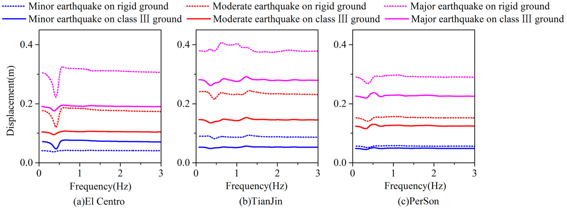
Figure 6 illustrates the peak displacements of the equipment top in the cases of the rigid ground and Class III ground. As shown in the figure, when the equipment’s frequency was f_e≈0.43 Hz, (i.e. close to the fundamental frequency of the HRS), the peak displacement of the equipment top reached a noticeable maximum under each ground motion. After the SSI effect was taken into consideration (Class III ground), the maximum peak displacement of the equipment top shifted toward lower frequencies. At this maximum point, f_e≈0.36 Hz, which means that the equipment’s frequency was approximately equal to the fundamental frequency of the HRS–soil subsystem in the case of Class III ground. The maximum peak displacements of the equipment top in different earthquake stages were considered and compared between the two cases. The results show that the maximum values during the minor earthquake, moderate earthquake, and major earthquake stages under El Centro ground motion in the case of Class III ground decreased by 25.7%, 18.3%, and 11.3%, respectively, compared with the corresponding values in the case of the rigid ground. The corresponding decreases under TianJin ground motion were 28.5%, 18.0%, and 9.0%, respectively. During the three earthquake stages under PerSon ground motion, the equipment top in the case of Class III ground experienced maximum peak displacements increased on 37.9%, 23.8%, and 13.4%, respectively, compared with those in the case of a rigid ground.

Figure 6.

Peak displacements of the equipment top in the cases of rigid ground and Class III ground.

The peak displacements of the structure top in the cases of the rigid ground and Class III ground are plotted in Figure 7. The peak displacement of the structure top reached an apparent minimum under each ground motion. These minimum points correspond to the maximum points shown in Figure 6. In other words, the peak displacement of the structure top reached its minimum when the equipment’s frequency was close to the HRS’s fundamental frequency in the case of rigid ground, or when it was approximately equal to the HRS–soil subsystem fundamental frequency after the SSI effect was considered. The minimum peak displacements of the structure top in the three earthquake stages were considered and compared between the two cases. Under El Centro ground motion, the minimum values during a minor earthquake, moderate earthquake, and a major earthquake in the case of Class III ground decreased by 12.7%, 9.6%, and 6.7%, respectively, compared to those in the case of the rigid ground. Under TianJin ground motion, the structure top showed minimum peak displacement decreases of 18.1%, 15.7%, and 10.8%, respectively, compared to those in the case of the rigid ground. Under PerSon ground motion, the corresponding decreases in the minimum peak displacement of the structure top were 8.7%, 6.3%, and 5.8%.

Figure 7.

Peak displacements of the structure top in the cases of rigid ground and Class III ground.

An analysis of the seismic responses reveals that after the effect of equipment–HRS–soil interaction was taken into account, the peak displacement of the equipment top exhibited a noticeable maximum while the peak displacement of the structure top had an obvious minimum. The equipment’s frequency at this point was close to the HRS’s fundamental frequency in the case of rigid ground or approximately equal to the HRS–soil subsystem’s frequency after the SSI effect was considered. The analysis above concludes that, after the effect of SSI on the equipment was considered, the peak displacements of the equipment top in the case of Class III ground tended to decrease from those in the case of a rigid ground under El Centro and TianJin ground motions but that tended to increase under PerSon ground motion. By contrast, the peak displacement of the structure top tended to decrease significantly when considered the SSI effect, indicating that the SSI effect enhances the structure’s safety in the event of an earthquake. As the earthquake intensity increased, the magnitude of a change in the structure’s minimum response tended to decrease, suggesting that the positive effect of SSI on the structure weakens with increasing earthquake intensity.

Conclusion

The interactive numerical computation was proposed to achieve a simulated process of RTSSTT which introduced an LNS model considering that the soil is not completely in nonlinear status under strong earthquakes. This study leads to the following conclusions:

1. The equation of motion for the equipment–HRS–LNS system was derived through a combination of the branch modal substructure and linear–nonlinear hybrid constraint modal substructure approaches, which is characterized by clear definitions, ease of use, and so on.

2. The interactive numerical computation process was successfully simulated by interactive numerical computation using MATLAB and ANSYS. The continuous reading and writing of data by the software provided computational data communication.

3. Compared to integrated finite element analysis, the interactive numerical computation method can significantly improve the computational efficiency while ensuring accuracy. This confirms that the application of LNS model can provide powerful technical support for nonlinear soil participating in analysis. And the interactive numerical computation method also offers an effective channel to compute and analyze complex equipment–HRS–soil systems.

4. When the equipment’s frequency was close to the fundamental frequency of the HRS in the case of rigid ground, or when it was close to the fundamental frequency of the HRS–soil subsystem after the SSI effect was considered, the peak displacement of the equipment top reached a noticeable maximum while the peak displacement of the structure top showed an obvious minimum. Given that the seismic responses of equipment and HRS will change substantially when the SSI effect is taken into account, it is necessary to investigate the seismic response of the whole equipment–HRS–soil system in the seismic design of high buildings.