Sage Journals: Discover world-class research

Abstract

This paper aims to investigate the aerodynamics including the global performance and flow characteristics of a long-shrouded contra-rotating rotor by developing a full 3D RANS computation. Through validations by current experiments on the same shrouded contra-rotating rotor, the computation using sliding mesh method and the computational zone with an extended nozzle downstream flow field effectively works; the time-averaged solution of the unsteady computation reveals that more uniform flow presents after the downstream rotor, which implies that the rear rotor rotating at opposite direction greatly compensates and reduces the wake; the unsteady computations further explore the flow field throughout the whole system, along the span and around blade tips. Complex flow patterns including the vortices and their interactions are indicated around the blade roots and tips. For further identifying rotor configurations, the rotor–rotor distance and switching two rotor speeds were studied. The computation reveals that setting the second rotor backwards decreases the wake scale but increases its intensity in the downstream nozzle zone. However, for the effect of switching speeds, computations cannot precisely solve the flow when the rear rotor under the windmill because of the upstream rotor rotating much faster than the other one. All the phenomena from computations well implement the experimental observations.

Keywords

Shrouded contra-rotating rotor numerical computation sliding mesh vortex interaction flow unsteadiness

Introduction

The requirements of miniaturization and high hover performance of unmanned aerial vehicles (UAVs) result in a very low working Reynolds number for rotors, which is nearly close to the flight Reynolds number regime 10,000 to 50,000.¹ Under such low Reynolds number, the rotor’s flow field and aerodynamics are easily affected by the turbulence intensity and surface roughness, which is distinguished with the conventional rotor (Reynolds number is bigger than 10⁶). Its viscosity effects and unsteady effects tend to be more significant, compared to the flow passing through a conventional rotor.^2–4 It easily brings the aerodynamic problems such as laminar separation bubble, nonlinear effect of lift coefficient, and static delay effect, which consequently degrade the aerodynamic performance of the rotor. Although the researchers tried to optimize the airfoil for the low Reynolds number flight and already made some achievements on improving the rotor efficiency, the figure of merit (FoM, currently maximum is about 0.6) is still lower than that of a conventional rotor (currently maximum is about 0.8).^5,6 Therefore, further investigations on the lift-enhancement are urgently required. One of possibilities is the unconventional lift configuration.

The configuration–shrouded contra-rotating double rotor (i.e., shrouded double rotor (SDR)), which consists of two contra-rotating coaxial rotors and a shroud with a cross-sectional profile as an airfoil, was identified to improve the hover capability of MAVs. Compared with free rotors, it was proved that putting rotors into a shroud with the same axis as the shroud can effectively increase the hover performance.^7–10 There have been researches for larger ducted counter-rotating rotor used on the turbomachinery which works in a relatively high Reynold number.¹¹ However, operating in a low Reynolds number, such configuration still has many aerodynamic problems such as the transition from laminar flow to the turbulent flow at the inlet, which can aggravate the unsteady features of the flow.^12,13 Meanwhile, due to the configuration, the interactions among different components result in a very complex flow. Therefore, in order to reveal the potential aerodynamics and flow features, computations become necessary as a supplementary approach to current experiments.

This paper aims to develop reliable numerical methodology to study the topology of the flow which takes place among different components under the viscous effects. This analysis supports the conclusions revealed by the experiments conducted by Chao Huo.¹⁴ The SDR model used in the experiments consists of a 180-mm-main-inner-diameter shroud and two-bladed rotors installed at the same axis. Huo et al.¹⁰ made the early experiments regarding the shroud model, which was proposed by the two-dimensional axisymmetric simulations.¹⁵⁵ The contra-rotating rotor was specifically designed for shrouded systems by Drela and Youngren¹⁶ with nonzero circulation at the blade tip. The detailed geometrical parameters of both shroud and contra-rotating rotor can be found in Huo et al.¹⁴

In the study by Huo et al.,¹⁴ the experimental test bed was designed to understand the flow physics and the interaction between different components of the shrouded contra-rotating rotor, as shown in Figure 1. The test bed can not only test the individual performance parameters such as thrust and torque, but also measure the evolution of aerodynamic variables that characterize the flow passing through the shroud, such as total and static pressure. From the results, it is found that both the FoM of contra-rotating rotor and the system power loading are improved by the shroud inclusion. Compared to free rotors, the strong suction peak formed on the shroud leading edge by a 65% increase in mass flow, allowing the shroud to contribute up to 56% of the total thrust.

Figure 1.

Test bed configuration (a) and simplified working schematic (b).¹⁴

The shroud presence increases the complexity of the flow due to interactions between the shroud and rotors. Focusing on the shrouded single rotor (SSR) system, Akturk and Camci made a thorough investigation on system design issues, global performance assessments, and the flow field such as the tip clearance flow through both experiments and computations.^17–20 A custom-developed rotor disk flow model was used to accelerate the viscous flow computations. A prescribed static pressure rise was applied across the rotor disk for a time efficient simulation. This computational method was proved by the experiments that it can be highly effective and time efficient for SSR. Regarding the shrouded contra-rotating rotor, Ahn and Lee also developed a computational model which applied actuator disk for an axisymmetric ducted fan system.²¹ Actuator disk is considered as an infinite thin disk with a certain pressure jump on both sides of the disk to replace the real rotor. Their results showed increasing diffuser angle of the duct improved the propulsion efficiency of the ducted fan system, while the inlet geometry had little effect on it. Since 2003, in ISAE France, the department of the aerodynamic, propulsion, and energy has conducted many studies on both experiments and computations for shrouded contra-rotating MAVs. Thipyopas et al. tested the hover performance and horizontal forward flight characteristics of a short-shrouded coaxial configuration applied on MAV “Satoorn.”^22,23 Their study indicated that the optimization happens when both rotors produce approximately identical thrust, almost same pitch angle, and the rear rotor rotating relatively faster than the upper rotor. Parallel to their experiments, Grondin et al. made numerical simulations to calculate the flow field around the shroud.²⁴ An actuator disk method was also used. The results agree well on total lift induced by the mass flow through the rotor, but power comparisons show great divergences due to disregard for swirl flow and rotor losses. Currently, Han and Xiang compared the performance between a microscale shrouded coaxial rotor and an open coaxial rotor through both tests and computations.²⁵ Their work mainly focused on the system global performance and the influence of some typical design parameters.

Compared with SSR, the shrouded contra-rotating rotor involves more complex flow interactions, not only between the shroud and the rotor, but also between two rotors. There are limitations for current computations which mostly used actuator disk for SDR system. The actuator disk method ignores the number of blades, the rotation effect, the flow viscosity over the rotor surface, and the interactions among different components. Therefore, the real rotors with rotating motions must be considered in order to explicit the aerodynamic performance and flow characteristics of the SDR system. Different from most present works, this paper focused on the development of a fully unsteady 3D Reynolds-Averaged Navier-Stokes (RANS) computation methodology which concerns on the actual double rotor configurations. First, the paper discussed different multiple reference frame methods—mixing plane and sliding mesh, and compared two definitions of computational fields. Based on a well-defined structure mesh, the computational methodology was validated by our experiments; the aerodynamic performance and flow characteristics of a SDR system were further analyzed for implementing current experiment results through numerical computations. To identify and further improve the double rotor configuration, the effects of rotor–rotor distance and switching speeds were also explored numerically.

Methodology of 3D computation

With regard to the experimental work,¹⁴ the best performed SDR system with the upstream rotor located at 80 mm from the inlet and inner rotor distance (IRD) of 20 mm was also chosen in the computation work. As the SDR system involves two rotors rotating at the opposite direction, it needs two reference frames to define each rotating motion, as shown in Figure 2. The SDR system is separated into four parts. On the interfaces between rotating zones, there are usually two methods—mixing plane and sliding mesh, which can treat the transformation of vector quantities. Obviously, the flow at the boundary between adjacent zones of rotor–rotor (R/R) is not radially uniform, and the sliding mesh is then a general approach for such case. Based on a final, time-periodic solution, the data should be time averaged during one period for the steady performance analysis of the system. Comparing with sliding mesh, the mixing plane method is used only for calculating steady flow, but it sometimes would be more complicate if the flow is not radially uniform. In this paper, sliding mesh method was chosen. Hence, the shroud upstream and downstream zones should be further adjusted according to the requirement of the boundary conditions.

Figure 2.

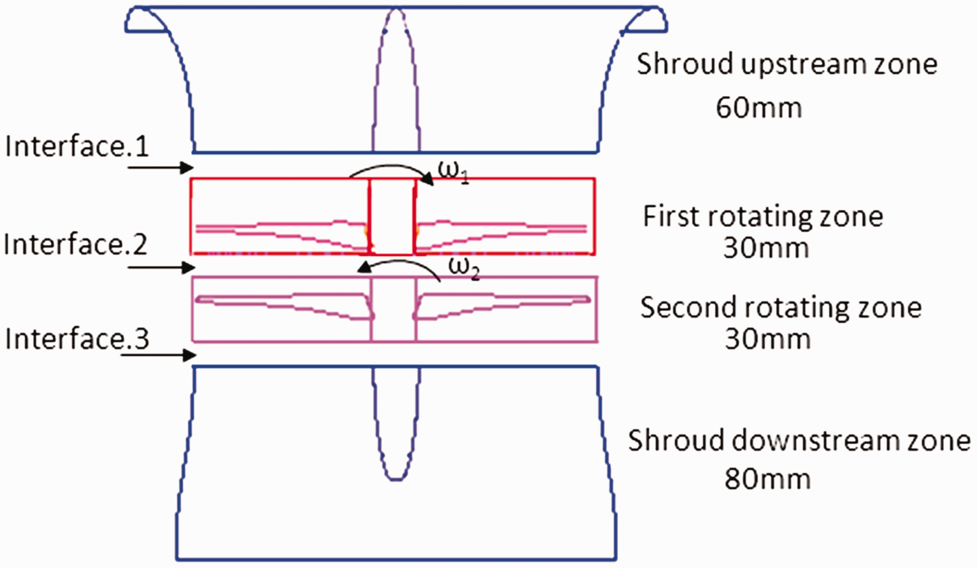
Scheme of zone separation and interfaces.

Computational field and boundary conditions

The computational field is composed of the air entrance, the rotor zone, and the exit downstream zone. The boundary condition “total pressure” was imposed at the inlet. However, at the geometric inlet, the flow accelerates near the leading edge due to the shroud lip curvature and therefore is not uniform. Different definitions of the inlet geometric parameters were discussed in Jardin et al.,¹³ which proposed a homokinetic normal inlet surface model to ensure the uniform flow features at the inlet boundary. Therefore, in this work, a semispherical geometry which is big enough with a radius of 2.5 times rotor radius Rr was introduced on the top of the shroud geometric inlet. For the downstream zone, the “static pressure” outlet boundary condition brings a trouble to define the location where the exit is, because the turbulence is significant at the mixing flow boundary of the exhaust flow and the ambient flow, which can easily induce a reversed flow. Therefore, the computational downstream domain was firstly considered as the shroud nozzle. Meanwhile, since the effect of the outlet imposition is not sure, another computational field was defined as a truncated cone shape to allow the uniform flow features at the nozzle exit. These two-defined corresponding computational zones for air expanding will be further analyzed through the computations.

Two definitions of computational fields with correspondent boundary conditions are given in Figure 3. For the computational field with an extended downstream truncated zone, in order to avoid the reverse flow which might cause nonphysical phenomenon, a very small velocity of 0.5 m/s was imposed on the top and side surfaces of the truncated zone.

Figure 3.

Boundary conditions and computational fields without (a) and with (b) downstream cone.

Mesh

Based on the computational fields defined above, structured meshes were made through ICEM separately for upstream zone, two rotating zones and downstream zone, seen in Figure 4. For the rotating domains, as the effects of the boundary layer and the turbulence have to be revealed, two “O” grids were used to refine the mesh on the shroud wall and the hub. Meanwhile, due to the sharp shapes of the leading edge and the trailing edge at the blade tip, “Y” grid was used to avoid the mesh distortion. Totally, the cells used are approximately 6 million elements with a Y+ controlled lower than 5 around the wall and the blade.

Figure 4.

(a) Mesh of the upstream zone, (b) Mesh of the downstream zone and (c) Block and mesh of the rotating zones.

Numerical models

Some basic characteristics of the SDR system such as flow compression and turbulence should be firstly identified. For SDR system in this work, the maximum Mach number at the blade tip is about 0.25 under the condition of maximum rotational speed of 9000 r/min and blade radius of 0.089 m. The flow can be thus considered as incompressible. Meanwhile, based on the characteristic velocity of 10 m/s provided by experiments and the characteristic length of 200 mm (correspondent to the shroud length), the system Reynolds number and blade Reynolds number are calculated to be about 85,000 and 40,000, respectively, which are much larger than 3000—the separation for turbulent and laminar flow. The flow is undoubtedly turbulent.

Comparing with other turbulence simulation methodologies such as Large Eddy Simulation (LES) and Direct Numerical Simulation (DNS), unsteady RANS is more efficient and has less requirements for the mesh. Therefore, with the commercial code Fluent,²⁶ a fully steady 3D RANS computation was firstly conducted. Then its solution was applied as an initial condition input for unsteady RANS (URANS) simulations. A “pressure-based” solver and Spalart-Allmaras (S-A) turbulent model were chosen. Due to the huge amount of mesh cell number, S-A turbulent model is economic in terms of time cost and computation resource. Meanwhile, it was designed specifically for aerospace applications involving wall bounded flows. S-A turbulent model is known to have good results for boundary layers exposing adverse pressure gradient. It is suitable for mildly complex external and internal flows and boundary layer flows under pressure gradients. A coupled scheme was used for the pressure–velocity coupling equation and the spatial discretization recommends using the scheme of the second-order upwind. The solution of the computation was considered “converged” when the residual is in the order of 1.0e–6 and a regular periodic change of one typical quantity such as lift coefficient Cl presents.

Validations

The computational methodology was firstly validated by our experiments.¹⁴ One main objective of the experiments was to explore the aerodynamics of the micro shrouded contra-rotating system. At a certain range of rotational speed, the global performance such as thrust, torque, and power, the pressure distributions along the shroud wall, and the total and static pressure fields at several selected longitudinal stations of the system were explored by experiments. To further enhance the ability of a given shroud to aspirate the air, various rotor speeds and different rotor locations were tested to examine the shroud local aerodynamic effects through both wall pressure and field pressure measurements. Some results obtained by those tests were applied to validate the simulation in this paper. The detailed information about the experimental setup, program, and data can be found in Huo et al.¹⁴

Comparison between two computational fields

The two computational fields were calculated under the contra-rotational speed pair N₁=N₂=6000 r/min. In order to speed up the computations, the 3D computation with sliding mesh method was started with a relatively large time step 5.55 × 10⁻⁴ s. At each step the system rotates 20°. This was used in the first five circles until the periodically stationary solution appears. Then a smaller time step 5.55 × 10⁻⁵ s which allows the system to rotate 2° was used to obtain more precise solutions. For the first computation, when a stable periodic solution appears, the time step was changed to an even smaller one 2.78 × 10⁻⁵ s. Comparing two small time steps 5.55 × 10⁻⁵ s and 2.78 × 10⁻⁵ s, the periodic solution does not show any difference. Therefore, the time step 5.55 × 10⁻⁵ s was chosen as the one which can obtain the precise solutions. As shown in Figure 5, based on the final periodic revolutions independent on time, the time-averaged solutions were calculated during one period.

Figure 5.

The solution of Cl with time.

Table 1 shows that the mass is conserved at the inlet and exit for both computations. Compared to the computational field without nozzle downstream zone, the computational field with extended zone can obtain the mass flow more than 1%. This is caused by the ambient pressure on the actual nozzle exit, which affects the upstream flow condition. This should be further identified through a detailed analysis of the result.

Table 1.

Mass flow of the computations with different computational fields.

	Mass flow (kg/s)
Passages	Without downstream zone	With downstream zone
Inlet	0.3307	0.3341
Nozzle exit	0.3306	0.3341

Figure 6 presents the mean static pressure distributions on the symmetric surface in the downstream of the rotor for two computational fields. It should be noticed that the “mean” data showed in the figures is the time-averaged solution of unsteady computations. Figure 6 shows that for the computational fields without an extended downstream zone, the imposition of an ambient pressure on the nozzle exit leads to a movement of the relative zero pressure to the position parallel with the hub. Meanwhile, the computational field with an extended downstream zone has a relatively lower pressure distributed at the exit.

Figure 6.

Mean static pressure on the shroud downstream surface for computations without downstream zone (a) and with downstream zone (b).

Through extracting the data on a specific line 20 mm up from the nozzle exit, Figure 7 shows the comparisons on the mean static pressure between the calculations of two computational fields and experiments. In Figure 7, there are two sets of experimental data: one is from the static pressure test on the axial station by static pressure probe; the other one is from the shroud wall pressure test by the pressure transducers. It presents that the static pressure coefficient from the computation with a downstream extension zone is closer to the experimental date, compared to the Computational Fluid Dynamics (CFD) results without a downstream zone. However, the difference between CFD and experiments becomes evidently when close to the shroud wall. This is due to the pressure probe used in the test. The probe modifies the local flow when it is close to the shroud wall, the so test precision near the wall is thus decreased.

Figure 7.

Comparison between computations of two computational fields and experiments. Exp: experiments; CFD: Computational Fluid Dynamics.

Therefore, comparing with the computation in which the pressure boundary is imposed directly at the actual shroud exit, globally the computation with an extension of the downstream zone shows a more similar trend of static pressure radial distribution with experiments. Their slight difference around the major radial positions basically comes from the mass flow generation, which will be explained in the next section. The computational flow field with an extension downstream zone of the nozzle was therefore chosen for the following computations and analyses.

Validation on the final numerical methodology

Based on the computations of the computational field extended in the downstream, this section aims to validate the computation through experiments. A suitable reference for the validation should be decided in advance.

According to the actuator disk theory, the pressure jump △P formed on both sides of the rotors can be used as a function of rotors to generate a mass flow and quantify the rotor thrust (F_R=△P/A_R), while the shroud performance greatly depends on the mass flow rate $\dot{m}$ . The system behaviors are thus basically steered by these two variables △P and $\dot{m}$ . However, these two parameters have different relations with the rotational speeds, as shown in Figure 8, which gives multiple possibilities to choose a reference for the validation of 3D computations. Furthermore, Figure 8 shows the cases at P.1 and P.2 have the same rotational speeds but generate different mass flow ${\dot{m}}_{1}$ and ${\dot{m}}_{2}$ . Comparing the cases at P.2 with the one at P.3, they are in different speed levels but generate the same mass flow. Similar comparisons among those three points on the relationship between the rotational speed and the pressure jump can be derived. Therefore, both the rotational speed and the mass flow were chosen as references for validations in this work.

Figure 8.

Pressure jump △P versus mass flow $\dot{m}$ for different iso-speeds.

Validations on the global performance parameters

Table 2 gives an overall view on the global performance comparisons between CFD and experiments under two references: one is the same rotational speed 6000 r/min; the other is almost the same mass flow around 0.326 kg/s generated by a rotational speed pair of 5790 r/min. Here it should be mentioned that the same mass flow as experiments is quite difficult to be obtained in terms of the computation, as it requires huge iterations. Globally, under the same mass flow input, the computation provides quite consistent solutions with experiments. The differences on the various performance parameters between CFD and experiments are all lower than 5%. On the contrary, comparisons of the same rotational speed show bad agreement on the performance. The difference on mass flow 3.1% brings a large variation on the shroud thrust of 16.9%. The upper rotor generates 15.5% thrust more than in experiments due to a possible blade distortion, which cannot be considered in CFD.

Table 2.

Comparison on global performance between CFD and experiments.

Performance	Ref. N	Ref. $\dot{m}$		Ref. N	Ref. $\dot{m}$
Performance	3D CFD	3D CFD	Exp	Var (%)	Var (%)
$N_{r 1}$ (r/min)	6000	5790	6000	0	3.3
$N_{r 2}$ (r/min)	6000	5790	6000	0	3.3
$\dot{m}$ (kg/s)	0.336	0.329	0.326	3.1	0.9
$F_{r 1}$ (N)	0.641	0.558	0.535	15.5	4.3
$F_{r 2}$ (N)	0.793	0.723	0.76	4.4	−4.8
$F_{sh}$ (r/min)	1.79	1.6	1.53	16.9	4.5
$Q_{r 1}$ (N.m)	0.0168	0.0152	0.0148	13.4	2.7
$Q_{r 2}$ (N.m)	0.0194	0.0179	0.0184	5.6	−2.7

CFD: Computational Fluid Dynamics.

Validations on the flow field

Figure 9 presents the distributions of total pressure coefficients along the radial positions on two chosen axial planes upstream (20 mm from the inlet) and downstream (40 mm from the rear rotor) rotors for both computations and experiments. We can see, before two rotors, that the total pressure at two rotational speeds is almost the same. In the downstream rotors, due to a greater power input, the flow at 6000 r/min provides a greater total pressure than the one at 5790 r/min. In general, both computations can well solve the flow. And the computation with the same mass flow can provide a more similar solution with the experimental data in the downstream rotors, compared with the computation with the same speed 6000 r/min. It should be noticed that a relatively big difference always appears at the positions near to the shroud wall where r/R_max is close to 1. The effect of the boundary layer is more significantly in computations. The reduction of total pressure near the wall is more evident on the plane before rotors. This may be due to two aspects: first, the application of turbulent model Spalart-Allmaras with one equation has relative lower precisions on solving the boundary layer; second, before passing the rotor passages, the flow has not been accelerated sufficiently and it behaves more like laminar, under which the flow is highly dominated by viscosity.

Figure 9.

Comparison of total pressure coefficient at different axial planes: 20 mm from the inlet (a) and 40 mm after the rear rotor (b). Exp: experiments; CFD: Computational Fluid Dynamics.

Similarly, Figure 10 shows the distributions of static pressure coefficients for both computations and experiments. Compared to the total pressure, the global consistence of the static pressure distribution especially at the axial planes after rotors is relatively worse. This might be caused by the complexity of the wake which decreases the precision on solving the static pressure. Obviously, comparing with the same rotational speed, the same mass flow input can provide more similar solutions on the static pressure as the tests. However, at positions near the shroud wall, there is great difference between computations and the experimental data tested by the static pressure probe. This is because the measurement precision is decreased when the probe is close to the shroud wall. Such problem does not exist in the static pressure tests by the shroud wall tubes connected to pressure transducers. Better agreement for computations is thus obtained with the data tested by the shroud wall tubes.

Figure 10.

Comparison of static pressure coefficient at different axial planes: 20 mm from the inlet (a) and 40 mm after the rear rotor (b). Exp: experiments; CFD: Computational Fluid Dynamics.

In general, the computation agrees the experiment better under the same mass input compared to the reference of rotational speeds. All the validations on the global performance and flow field indicate the computation can effectively work. The computation can be applied to explore the potential steady and unsteady characteristics in order to understand more about the system as a complementary approach for experiments.

Numerical explorations on system performance

For the analysis of the hover performance of the SDR system in the study by Huo et al.,¹⁴ there are limitations for current experiments: first, due to the limited space and strong flow interactions between rotors, the probe is hard to test the flow at the middle plane of two rotors. The flow characteristics between rotors are thus not clear; second, the experiment was actually two dimensional since it cannot take the radial component of the flow into account; third, the flow features revealed by experiments were still from a global view. The flow field was not explored in detail due to the limited test facilities and huge time cost. Therefore, in order to complement the experiments and provide a throughout understanding of the SDR systems, this section aims to explore the detailed flow characteristics of the SDR system through a full 3D numerical computation that was validated above.

Steady flow characteristics

To explore the flow development in detail, five isolated surfaces along the shroud axis were chosen at the same positions as the ones in experiments: four planes located 20 mm, 60 mm, 90 mm, and 140 mm from the inlet, respectively, and the outlet. In this section, the analysis on the aerodynamics of the system was based on the time-averaged solution of the unsteady computation. The flow passing on those surfaces complements the understanding of the system from the experiment.

Based on the time-averaged solutions, the radial distributions of the mean static pressure on five surfaces introduced above are presented in Figure 11. The mean static pressure distribution shows a smoothly decrease from the axial center to the shroud, and the negative pressure is formed over the entire inner surfaces of the shroud due to the flow acceleration. On the surface Y = 20 mm, the mean static pressure has the most significantly radial variation about 50 Pascal compared to other surfaces because of the greatest profile curvature near the entrance. The relatively low pressure continues to the upstream rotor. From the surfaces Y = 20 mm to 60 mm, the flow is depressed and accelerated by narrowing shroud passage, which leads to a further decline of the pressure. Through two rotors, the pressure is followed by a dramatical increment. On the surface at Y = 90 mm between the two rotors, the mean static pressure around the radial position 0.86 R_max dramatically decreases, which might be the loss caused by the tip vortex. This loss is quickly compensated by the contrary rotation of the rear rotor. It can be observed through the distribution on the surface Y = 140 mm, where there is no such great radial change between the tip and the hub. Obviously, more uniform flow presents after the rear rotor. At the outlet, the flow is slightly over-expanded and the static pressure is a bit lower than the ambient pressure.

Figure 11.

Mean static pressure radial distributions at different axial planes: (1) Surface 1 before rotors: L=20 mm; (2) surface 2 before rotors: L=60 mm; (3) surface 3 between rotors: L=90 mm; (4) surface 4 behind rotors: L=140 mm; (5) surface 5 outlet: L=200 mm.

Figure 12 shows the mean total pressure distributions. Until the upstream rotor, the flow is quite uniform except the region around the shroud boundary layer and the hub, where the total pressure is dramatically decreased and lower than zero. The viscosity causes a great pressure loss near the wall. After the first rotor, the losses become more pronounced near the shroud wall and the hub which is mainly caused by the vortex. The detail information about the flow pattern will be explored in the following sections. Behind the rear rotor, the total pressure reaches the highest in the main region due to the power input by the rotor rotation. At the outlet, the pressure around the shroud and hub is close to the ambient pressure, which implies the definition of the computational downstream zone is reasonable.

Figure 12.

Mean total pressure radial distributions at different axial planes: (1) Surface 1 before rotors: L=20 mm; (2) surface 2 before rotors: L=60 mm; (3) surface 3 between rotors: L=90 mm; (4) surface 4 behind rotors: L=140 mm; (5) surface 5 outlet: L=200 mm.

Along the whole shroud passage, the flow development can be observed in Figure 13. The rotor rotation aspirates the flow and accelerates it at the entrance due to the shroud profile curvature. The axial velocity is uniform in the main region but decreases near the wall due to the viscosity. After the double rotor, the nozzle diffuser expands the flow and thus the axial velocity is decreased.

Figure 13.

Axial velocity on the symmetric surface.

Typical unsteady flow patterns

As introduced at the beginning of the paper, the low Reynolds number makes viscous effect and unsteady features of micro shrouded rotors significantly, which can greatly attenuate the rotor performance. To further identify the performance of the SDR system, this section aims to explore the typical unsteady flow patterns of the SDR system from following aspects: tangential velocity, the flow along the span, and the flow at the blade tip. The solutions at four different times which equally divide one period (0.0025 s) were presented in the analysis of the unsteady flow.

Tangential velocity

The component of velocity—tangential velocity is a typical quantity to characterize the rotating motion of the flow. On the three selected iso-surfaces from the upstream to the downstream rotors, Figure 14 shows the tangential velocity distribution during one period.

Figure 14.

Tangential velocity distributions at different axial planes: (a) Surface in the upstream rotor: L=60 mm. (b) Surface between two rotors: L=90 mm. (c) Surface in the downstream rotor: L=140 mm.

As shown in Figure 14, a circumferential distribution no longer exists in unsteady flow. For all the surfaces, it can be observed that the relatively great tangential velocity is distributed around the blade and follows the rotation of the blade during the whole period. Without the effect from the upstream rotor rotation, on the surface Y = 60 mm the tangential velocity is almost around zero except a small tangential velocity presenting around the blade. On the surface between two rotors, the flow is accelerated under the rotation of the upstream rotor. The tangential velocity near the blade becomes significant. However, it is followed by a dramatical decrement on the surface Y = 140 mm. Comparing all the stations, the most evidently tangential velocity is formed at the surface just after the upstream rotor. This is modified by the rear rotor which rotates in the opposite direction, seen in Figure14(c). It should be noticed that another region close to the hub has strong tangential component of the velocity. It implies that a complicated flow pattern not only exists around the blade tip but also the blade root.

Flow along the span

To understand the flow between rotors, Figure 15 presents the vorticity contours at three spanwise stations 0.2 Rr, 0.75 Rr and 0.96 Rr at one specific time of 4/4T, when the upstream rotor rightly overlaps the downstream rotor and the interactions between two rotors is relatively strong. At the span of 0.2 Rr, both rotors have a trailing vortex. The flow of the trailing wake from the upper rotor is strongly engaged into the vortex generated by the lower rotor. Especially for the downstream rotor, the wake is extended with a downwash velocity. At the position of 0.75 Rr, the trailing vortices from both rotors are separated into two. Comparing to the location 0.2 Rr, the flow passing through the downstream rotor at 0.75 Rr suffers little influence from the upstream one. At the span position of 0.96 Rr, the vortex impinging into the vortex of the downstream rotor appears again. The vorticity magnitude becomes significant due to the wake in the downstream shear region and the effects from the shroud wall boundary layer. The strong vortices and their interactions between rotors are the main reasons that cause the total pressure loss around the blade tip and root, as shown in Figure 12.

Figure 15.

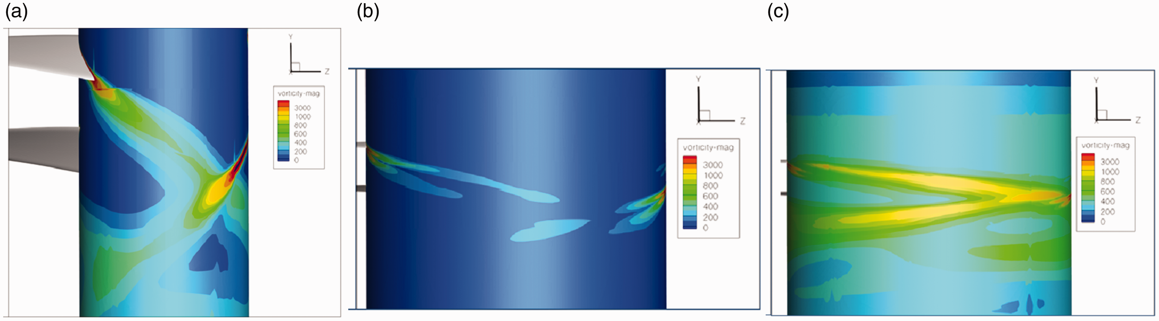
Vorticity of upstream and downstream rotors at different spanwise locations (4/4T): (a) 0.2 Rr; (b) 0.75 Rr; and (c) 0.96 Rr.

Flow at the blade tip

Due to the variation of velocity along the span, a pressure gradient is formed on the blade surface. The pressure on the suction surface differs from that on the pressure surface greatly so that tip flow generates. For unsteady flow, the vortex generated in the system was indicated to be one of the critical sources resulting in an aerodynamic loss.²² Therefore, it is important to clear such vortex pattern, position and scale for the SDR system.

Figure 16 indicates the helicity on several surfaces along the blade chords of both upstream and downstream rotors during one period. For both rotors, typical vortex structures around the blade tips have quite similar features: In general, the tip vortex grows from the leading edge to the trailing edge. Due to the flow separation developed along the chord direction, a complex tip vortex is produced and a secondary vortex is generated on the suction surface. Meanwhile, with the vortex development along the chord, the secondary vortex is crashed into the tip vortex more and more. Finally, they are formed into one with a relatively large scale. Comparing the vortex around both blades, because the downstream rotor rotates under the effect of the swirl flow produced by the upstream rotor rotation, globally the intensity of the downstream vortex is greater than the one formed at the upstream blade tip. To view the flow on two rotors separately, it can be observed that for upstream rotor, the vortex structures have no obvious change during a whole period. This implies that the blade is hardly affected each other since the rotor only has two blades. Furthermore, the upstream rotor is not affected by the downstream rotor either, which is different from the downstream rotor. During one period, although the vortex pattern keeps quite similar, the vortex intensity varies with time. At the time of 4/4T (see Figure 16), when the upstream rotor rightly overlaps the downstream one, the downstream tip flow is under the strongest influence from upstream flow, the vortex intensity is greatest compared to other moments.

Figure 16.

Streamwise helicity contours at blade tips of upstream rotor (a) and downstream rotor (b).

As introduced above, the vortex is one of the main sources causing the aerodynamic loss. One of the typical vortexes is blade tip vortex. For open rotor systems, the tip vortex can cause a big pressure loss and then decrease the rotor efficiency. However, the shrouded system can effectively minimize the loss because the shroud can limit the development of the tip vortex. Figure 17 gives a good view for the vortex structure around two blade tips at the time 4/4T. It can be seen that two main tip vortices are formed and expanded along with the rotations. A certain flow with downwash velocity from the tip vortex of the upstream blade tip detaches the downstream blade suction surface and then directly engages into its tip vortices.

Figure 17.

Streamlines around the upstream and downstream blade tips at the time 4/4T

Effect analysis of the coaxial rotor configurations

The experiments in Huo et al.¹⁴ analyzed the effects of rotor locations and switching speeds in terms of the global performance as well as the static and total pressure distributions along several axial shroud stations. To provide a deep view on the effects of different rotor configurations, the computations in this section focus on the analysis of the unsteady flow field of different rotor configurations.

Inner rotor distance

Correspondent to the experiments, two same rotor locations SDR80-40 and SDR80-20 were chosen. SDR80-40 means the SDR with the first rotor located 80 mm from the inlet and the second rotor located 40 mm from the first rotor. The same is for SDR80-20, which has a different IRD 20 mm. The computations were made at the same rotational speeds 6000 r/min as the experiments for the convenient of comparisons.

Table 3 shows the comparisons on different performance parameters between computations and experiments. It can be observed that, taking the rotational speed as a reference, the computations usually obtain more mass flow compared with experiments. From the validations of the computation introduced in Validations section, the difference can be decreased by using the reference of the mass flow. From Table 3, the same conclusion as experiments can be observed that the SDR system performance is not sensitive to IRDs. With two different IRDs, the differences are quite small concerning the thrust performance and rotor efficiency—FoM.

Table 3.

Comparison between computations and experiments.

Performance	CFD	Experiment	CFD	Experiment
Performance	SDR80-40	SDR80-40	SDR80-20	SDR80-20
Mass flow (kg/s)	0.333	0.324	0.336	0.326
Ft (N)	3.209	2.815	3.224	2.825
Fs/Ft (–)	0.54	0.54	0.56	0.54
FoM (–)	0.68	0.66	0.68	0.67

CFD: Computational Fluid Dynamics.

Since the upstream rotor affects greatest the downstream rotor when two rotors overlap, the comparison on the flow fields of two IRDs is hence made at the time 4/4T. Comparing the vorticity developed in the axial flow direction at the radial position 0.8 Rr of two IRDs in Figure 18(a), it is evident for short IRD 20 mm that the wake of the upstream rotor blade is greatly engaged into the downstream one. Such interaction becomes weaker with a larger IRD 40 mm. However, the larger IRD allows the wake evolve longer. The intensity of vortex and the space between rotors for vortex development balance their impact on the system performance.

Figure 18.

Axial vorticity at radial surface 0.8Rr of SDR80-20 (a) and SDR80-40 (b).

The typical vortex or wake usually occurs not only between rotors but also in the downstream rear rotor. Figure 19 shows the vorticity distribution on the symmetric surface in the downstream rear rotor. Three main wake structures can be observed around the end of the hub, the shroud trailing edge, and the downstream free flow, respectively. Globally, the intensity of the wake for larger IRD of 40 mm is stronger than the one for shorter IRD of 20 mm, while the wake scale of the system with IRD = 40 mm is smaller. The wake with stronger intensity can lead to a greater loss, but the loss can be restricted by a shorter IRD. Therefore, similar with the aforementioned analysis for Figure 18, different IRDs cannot lead to a great difference on the system performance.

Figure 19.

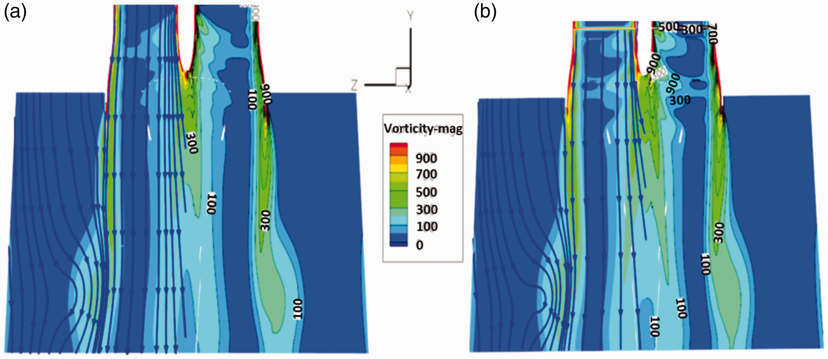
Streamlines and vorticity contour at symmetric surfaces of SDR80-20 (a) and SDR80-40 (b).

Switching speeds

From the experiments,¹⁴ switching speeds means exchanging the rotational speeds of two rotors, which can affect the system performance. The experiments indicated that the systems with two rotational speeds switched show a general similar performance. However, the optimal performance is always found for the system with the upstream rotor rotating more slowly than the downstream rotor. To explore the potential physical principles behind this phenomenon, two pairs of rotational speeds R1 = 6000 r/min, R2 = 9000 r/min (6000–9000) and R1 = 9000 r/min, R2 = 6000 r/min (9000–6000) were chosen for computations as same as experiments.

Table 4 shows the comparisons between computations and experiments at two rotational speed pairs. Unfortunately, the results of computations show an opposite conclusion: the system performance benefits from the rear rotor rotating at a lower speed than the upstream one, which allows the system aspirate more mass flow. The greatest difference occurs on the rear rotor performance with the rotational speed 9000–6000. Since the mass flow obtained by the computation is similar with the experiment, it means the rotors have similar inflow conditions at the inlet. The main reason for the difference is thus from the flow condition on the rear blade itself which results in different thrust and torque generations. Under the influence of the upstream rotor rotating at an extremely high speed, the rear rotor almost behaves like a windmill, under which the velocity angle is far from the perfect incident one. At this situation, the computation is probably cannot so precisely capture the flow deterioration and thus deviates from the experiment.

Table 4.

Comparison between computations and experiments for switching speeds.

Performance	CFD		Experiments
N₁–N₂ (r/min)	6000–9000	9000–6000	6000–9000	9000–6000
Mass flow (kg/s)	0.426	0.432	0.431	0.422
F_t (N)	5.165	5.340	5.083	4.685
F_R1 (N)	0.33	1.84	0.26	1.76
F_R2 (N)	1.96	0.54	2.04	0.31
P_R1 (Watt)	7.36	39.23	9.23	39.62
P_R2 (Watt)	41.38	10.34	42.44	9.17
F_s/ F_t (–)	0.56	0.55	0.55	0.56
FoM_R1 (–)	0.63	0.67	0.40	0.61
FoM_R2 (–)	0.67	0.74	0.68	0.47

CFD: Computational Fluid Dynamics.

Conclusions

To explore the detailed flow characteristics, taking the SDR used in the experiment as a reference, the paper conducted a full 3D RANS numerical computation. Instead of the actuator disc which is usually used as the simplicity of actual rotors, the computation in this work included the real double rotor with the contra-rotating motion for exploring not only the global performance, but also the detailed flow characteristics of the SDR system. Focusing on the rotor configurations, the effects of IRD and switching speeds were also analyzed through computations for further optimizations. The main conclusions are obtained as follows:

Through validations by the experiments under two chosen references as mass flow and rotational speeds, it indicates that the computation using sliding mesh method and a computational field with an extended downstream nozzle zone can effectively work. It can probably solve the flow passing through the SDR system.

Based on a time-averaged solution of unsteady computations, the 3D computation reveals the steady flow characteristics: in view of the mean static and total pressure, the flow suffers losses from the viscosity of the wall boundary and the vortex. Compared to the upstream flow, the downstream flow after the rear rotor shows more uniform flow features, which implies that the rear rotor turning at opposite direction greatly compensates the swirl produced by the upstream rotor.

The unsteady computation shows that a circumferential distribution no longer exists in unsteady flow. A strong tangential component of velocity which corresponds to a complex flow pattern follows the blade rotation and presents around both the blade tip and the root. The flow along the span further identifies that a strong wake interaction occurs around the blade tip and root. Particularly at the blade tip, two main structures of tip vortices were obtained by the streamlines. All of these features dominate the flow unsteadiness.

Setting the second rotor backwards decreases the wake scale but increases its intensity in the downstream computational zone, which balances their effect to the system performance. This implement the experiment conclusion: the system performance is not sensitive to the IRD although a shorter IRD 20 mm shows a better performance compared to IRD of 40 mm.

For the effect of switching speeds, the computation is not able to achieve the same phenomena as in experiments which concluded that the upstream rotor rotating at a lower speed compared to the rear rotor can obtain a better performance. The computation cannot precisely solve the complex flow of the rear rotor which is almost under the condition of windmill due to the fast rotating of the upstream rotor.

Footnotes

Acknowledgements

The authors also appreciate the technical support from Prof. Gressier and Prof. Barènes in the Propulsion Laboratory of the department of Aerodynamics, Energetics and Propulsion, Institut Supérieur de l’Aéronautique et de l’Espace.

Declaration of conflicting interests

The author(s) declared no potential conflicts of interest with respect to the research, authorship, and/or publication of this article.

Funding

The author(s) disclosed receipt of the following financial support for the research, authorship, and/or publication of this article: The project is supported by the Fundamental Research Funds for the Central Universities of China (No. 3102017OQD067 and No. 1191329723) and the National Natural Science Foundation of China (Grant No.11802244).

Appendix

References

Lowson

MV.

Aerodynamics of aerofoils at low Reynolds numbers. In: UAVs–14th unmanned air vehicle systems international conference, Bristol, UK, 12–14 April 1999.

Pines

Bohorquez

Challenges facing future micro air vehicle development.

J Aircraft 2006; 43: 290–305.

Bohorquez

Samuel

Sirohi

et al . Design, analysis and hover performance of a rotary wing micro air vehicle. J Am Helicopter Soc 2003; 48: 80–90.

Bohorquez

Pines

Rotor and airfoil design for efficient rotary wing micro air vehicles. In: American Helicopter Society 61st annual forum proceedings, Grapevine, TX, 1–3 June 2005.

Hein

Chopra

Hover performance of a micro air vehicle: rotors at low Reynolds number.

J Am Helicopter Soc 2007; 52: 254–262.

Grasmeyer

Keennon

MT.

Development of the black widow micro air vehicle. In: 39th Aerospace science meeting exhibit, Reno, NV, January 8–11, 2001, AIAA 2001-0127.

Barbely

Komerath

Novak

LA.

A study of coaxial rotor performance and flow field characteristics. In: AHS technical meeting on aeromechanics design for vertical lift, Fisherman’s Wharf, San Francisco, CA, 20–22 January 2016.

Pereira

Chopra

Effect of shroud design variables on hover performance of a shrouded rotor for micro air vehicle applications. In: AHS international specialists’ meeting on unmanned rotorcraft, Chandler, AZ, 18–20 January 2005.

Lee

Leishman

Rand

Design and testing of a ducted coaxial rotor system for application to a micro aerial vehicle. In: American Helicopter Society international 66th annual forum proceedings, Phoenix, AZ, 10–13 May 2010.

10.

Huo

Barènes

Gressier

Effect study of design variables on hover performance of long shrouded contra-rotating rotors. In: 46th Symposium of applied aerodynamics of rotating bodies, Orleans, France, 28–30 March 2011.

11.

Nouri

Danlos

Ravelet

et al . Experimental study of the instationary flow between two ducted counter-rotating rotors. J Eng Gas Turbines Power 2013; 135: 022601.

12.

Lakshminarayan

Baeder

JD.

Computational investigation of microscale shrouded rotor aerodynamics in hover.

J Am Helicopter Soc 2011; 56: 042002.

13.

Jardin

Grondin

Gressier

et al . Revisiting Froude’s theory for hovering shrouded rotor. AIAA J 2015; 53: 1836–1844.

14.

Huo

Barènes

, and Gressier

Experimental analysis of the aerodynamics of long-shrouded contrarotating rotor in hover.

J Am Helicopter Soc 2004; 60: 1–12.

15.

Huo

Barènes

Gressier

et al . Numerical study on parametrical design of long shrouded contra-rotating propulsion system in hovering. In: International conference on mechanical and aerospace engineering, Venice, Italy, 28–30 November 2011.

16.

Drela

Youngren

Axisymmetric analysis and design of ducted rotors. Report, Ducted Coaxial Rotor Design, ISAE Institut Supérieur de l’Aéronautique et de l’Espace, December 2005.

17.

Akturk

Camci

Experimental and computational assessment of a ducted-fan rotor flow model.

J Aircraft 2012; 49: 885–897.

18.

Akturk

Camci

A computational and experimental analysis of a ducted fan used in VTOL UAV systems. Department of Aerospace Engineering, Pennsylvania University, 2011.

19.

Akturk

Camci

Tip clearance investigation of a ducted fan used in VTOL UAVS, Part 1: baseline experiments and computational validation. In: Proceedings of ASME turbo expo turbine technical conference, 6–10 June 2011, Vancouver, Canada.

20.

Akturk

Camci

Tip clearance investigation of a ducted fan used in VTOL UAVs, Part 2: novel treatments via computational design and their experimental verification.

J Turbomach 2014; 136: 021005.

21.

Ahn

Lee

A computational method for the performance modeling and design of a ducted fan system. In: Baik DK (ed) Systems modeling and simulation: theory and applications. AsiaSim 2004. Lecture Notes in Computer Science, vol. 3398. Berlin: Springer, 2005, pp. 113–121.

22.

Thipyopas

Barènes

Moschetta

J-M.

Aerodynamic analysis of a multi-mission short-shrouded coaxial UAV: part I - hovering flight. In: AIAA applied aerodynamics conference, Honolulu, Hawaii, 18–21 August 2008.

23.

Thipyopas

Barènes

Moschetta

J-M.

Aerodynamic analysis of a multi-mission short-shrouded coaxial UAV: part II - translation flight. In: AIAA aerospace science meeting, Orlando, FL, January 4–7 2010.

24.

Grondin

Thipyopas

Moschetta

J-M.

Aerodynamic analysis of a multi-mission short-shrouded coaxial UAV: part III - CFD for hovering flight. In: AIAA applied aerodynamics conference, Chicago, IL, 28 June – 1 July 2010.

25.

Han

Xiang

et al . Experimental and computational analysis of microscale shrouded coaxial rotor in hover. In: International conference of unmanned aircraft systems (ICUAS), Miami, FL, USA, 13–16 June 2017.

26.

Ansys, Inc. Ansys user’s guide. Canonsburg, PA: Ansys, Inc, 2011.

Computational study on the aerodynamics of a long-shrouded contra-rotating rotor in hover

Abstract

Keywords

Introduction

Methodology of 3D computation

Computational field and boundary conditions

Mesh

Numerical models

Validations

Comparison between two computational fields

Validation on the final numerical methodology

Validations on the global performance parameters

Validations on the flow field

Numerical explorations on system performance

Steady flow characteristics

Typical unsteady flow patterns

Tangential velocity

Flow along the span

Flow at the blade tip

Effect analysis of the coaxial rotor configurations

Inner rotor distance

Switching speeds

Conclusions

Footnotes

Acknowledgements

Declaration of conflicting interests

Funding

Appendix

References