Sage Journals: Discover world-class research

Abstract

Linear rolling guide is increasingly being used as the transmission system in computer numerical control machine tools due to its high stiffness, low friction, good ability of precision retaining, and so on. The lubrication of rolling linear guide affects significantly its performance and hence monitoring the lubrication condition during its operation is of great importance. In this article, the relation between different lubrication conditions of linear rolling guide and their corresponding vibration signals is studied. Three lubrication conditions labeled as “Poor,”“Medium,” and “Good” are simulated to represent the actual working conditions. A data acquisition system is set up to acquire the vibration signals corresponding to different conditions. The wavelet packet decomposition is employed to perform time–frequency analysis of the raw signal, after which the energy distribution of the decomposed signals is extracted as the feature. Two linear rolling guides manufactured by different companies are used in the experiments. The results demonstrate that the relation between the energy distribution extracted from vibration signals and lubrication conditions follows a certain rule. A typical feedforward backpropagation neural network is used as the classifier to verify the effectiveness of energy distribution. The average classification accuracy of the network with energy distribution as input is more than 95%. The results show that the lubrication conditions can be characterized by “energy” hidden in the vibration signals and the energy distribution is an appropriate feature that can be used for fault diagnosis of linear rolling guide.

Keywords

Linear rolling guide vibration wavelet packet decomposition neural network fault diagnosis

Introduction

As an important element in the family of rotary motion–driven machine elements, linear rolling guide has been increasingly being used as the transmission system in computer numerical control (CNC) machine tools due to its high stiffness, low friction, good reliability, good ability of precision retaining, and so on.^1,2 In recent years, the growing demand for the high-speed and high-precision CNC machine tools leads to higher demands on the performance of the linear rolling guides.³ The lubrication of linear rolling guide affects significantly its performance. Specifically, poor lubrication will inevitably increase the friction and, consequently, exacerbate the wear of the rolling linear guide. Furthermore, poor lubrication causes abnormal vibration, accelerating the damage of the machine tool and affecting the quality of machining. In contrast, good lubrication reduces friction and noise while increasing the life and reliability of the linear guide. Therefore, monitoring and identifying the lubrication condition during the operation of the rolling linear guide plays an important role in terms of improving accuracy and life of the linear guide.

However, the lubrication condition can be hardly observed directly when the linear rolling guide is under operation. With the progress of sensor technology, data acquisition/storage techniques, and data processing algorithms, structural monitoring systems (SHMs) are increasingly being employed by industry.⁴ SHM employs sensors installed in the structures to monitor the signals that may convey the damage or fault information in the structures without affecting the normal operation of the machine.⁵ The commonly used signals for health monitoring and fault diagnosis include current,⁶ acoustic emission,⁷ transmission error,⁸ and vibration. Among various signals, the vibration signal is the most widely used in the rotary machinery systems such as rolling bears, gears, and ball screws. Monitoring the vibration signals has various advantages such as continuous as well as intermittent monitoring, that is, analyses can be performed without stopping the machine and problems can be identified before they become serious. In addition, the ease of use, sensitivity toward faults, less time consumption, robustness, wide available range and so on promote the widespread use of vibration signals.⁹ A previous study showed that 82% of health monitoring has been carried out using vibration signals.¹⁰ Sawalhi et al.¹¹ quantified the spall size of the rolling element bearings using vibration data analysis and obtained a satisfactory estimation size of the spall. Guo et al.¹² employed vibration signals acquired from ball screw nut to perform fault analysis of the ball screw support bearing.

After the acquisition of the raw signals, various signal processing and pattern classification techniques can be used for fault diagnosis. Fault diagnosis mainly contains two research contents as follows: the first is analyzing the raw signal and extracting features dynamically or manually that can distinguish different fault modes of the devices, for example, normal, outer race fault, inner race fault, and ball fault of a bearing; the second is mapping the extracted features to the corresponding fault mode based on classification techniques. There are various fault diagnosis approaches presented in the literature in the recent five years. Hu et al.¹³ proposed a systematic semi-supervised self-adaptable fault diagnosis approach, which allowed dynamically selecting the features to be used for performing the diagnosis. Lei et al.¹⁴ proposed a two-stage intelligent fault diagnosis method using unsupervised feature learning. The method first learn directly features from raw signals using an unsupervised neural network and then classify the health conditions based on the learned features through softmax regression. Dhamande and Chaudhari¹⁵ proposed a compound fault feature extraction method based on time–frequency method and verify the extracted features using three classifiers, that is, feedforward backpropagation (BP) neural network, support vector machine, and Naïve Bayes classifier. He and He¹⁶ proposed an optimized deep learning structure, large memory storage retrieval neural network, to implement the diagnosis of bearing fault. Zhong et al.¹⁷ proposed a three-stage diagnosis framework consisting of signal processing and feature extraction, fault diagnosis by a probabilistic ensemble method, and parameter optimization and performance evaluation. Mao et al.¹⁸ extracted features from vibration signals acquired in a bearing test rig provided by the Center of Intelligence Maintenance System (IMS) in University of Cincinnati. An online sequential prediction method based on extreme learning machine was proposed to classify the features extracted from the vibration signals. The validation results showed that three faults modes, that is, outer race, inner race, and ball fault, were identified with high diagnosis accuracy. Jia et al.¹⁹ proposed a local connection network (LCN) constructed by normalized sparse auto encoder (NSAE), namely, NSAE-LCN, for intelligent fault diagnosis. The method was validated using the vibration signals acquired from a gear and a bearing test rig.

From the recent studies on fault diagnosis that are reviewed above, we see that extracting features that convey the fault information is a key step. The features are normally extracted from the time, frequency, or time–frequency domain. Fourier transform is commonly used in analyzing the frequency contents of the signal. But it is difficult to analyze signals which have features coming in at different scales or resolution. Wavelet transform uses the joint time–frequency domain to characterize signals, which has an essential improvement over Fourier transform. However, wavelet transform only decomposes the low-frequency part (also called “approximation”) of the signal, while the high-frequency part (also called “detail”) is no longer decomposed. More specifically, the original signal is split into a first-level approximation and a first-level detail. The first-level approximation is further split into second-level approximation and detail, while the first-level detail is not split. This process can be repeated as many times as needed, but each time only approximation is decomposed. Therefore, the ordinary wavelet transform can well characterize the signals having low-frequency information as their main components but, for the signals containing lots of detailed information such as non-stationary vibration signal, it is not able to well decompose and characterize. Wavelet packet decomposition (WPD) was presented by Coifman and Meyer on top of orthogonal wavelet basis to overcome the above problem.²⁰ For WPD, in each level, both the approximation and the detail are decomposed. WPD is also known as sub-band tree structuring since the decomposition process can be characterized by a full binary tree. WPD provides finer decomposition of the detail (high-frequency) part of the signal, making it possible to perform local time–frequency analysis of the signals that contain medium- and high-frequency information as their main components. Due to its ability of processing high-frequency signals, WPD has been used in many applications such as fault diagnosis of non-stationary signals, feature extraction, and signal denoising. García Plaza and Núñez López²⁰ applied WPD to vibration signals. The packet feature extraction in vibration signals was applied to correlate the sensor signals to the measured surface roughness to realize roughness monitoring in CNC turning operations. Li et al.²¹ designed an online monitoring and fault diagnosis system for belt conveyors using WPD and support vector machine based on vibration signals. The energy for each frequency band is extracted as the feature. Ma et al.²² proposed a fault diagnosis method based on wavelet packet energy entropy and fuzzy kernel extreme learning machine. The method was verified through identifying three fault modes of rolling bearing. Bianchi et al.²³ employed WPD to analyze the acoustic emission signals acquired in a rail contact fatigue test. Fei et al.²⁴ used WPD to extract Shannon entropy from the vibration signals as the features for bearing fault identification.

It can be seen that fault diagnosis of mechanical systems such as gears, bearings, and ball screw have been well researched. But the literature regarding the online monitoring and fault analysis of linear rolling guide is insufficient. Being one of the most important factors that affect the machining precision, the lubrication condition of linear rolling guide under operation needs to be monitored online and, furthermore, the lubrication status identification needs to be researched, which is the motivation of this study. To our best knowledge, this is the first study to carry out research of fault diagnosis from online signals on the linear rolling guide. In this article, the mapping relation between different fault modes of linear rolling guide and their corresponding vibration signals is studied. The fault modes here refer to three lubrication conditions labeled as “Poor,”“Medium,” and “Good” in the actual working conditions. The WPD is employed to extract features from the time–frequency domain of raw vibration signals. More specifically, the energy reconstruction algorithm is used to reconstruct the decomposed signals, forming energy distribution as the feature vector. To verify the effectiveness of the proposed feature, a typical feedforward BP neural network is employed. The article is organized as follows. Section “Feature extraction using WPD” details the WPD-based energy extraction algorithm. In section “Case study,” a case study is carried out. Three different lubrication conditions of the linear rolling guide marked as “Poor,”“Medium,” and “Good” are simulated by removing the original lubricant, lubricating using oil, and lubricating using grease, respectively. The vibration signals corresponding to the three lubrication conditions are acquired. In section “Results and discussion,” the relation between the vibration signal and the corresponding lubrication condition is studied using the WPD-based energy extraction algorithm. In addition, to verify the effectiveness of the feature, a typical feedforward BP neural network is employed as the classifier. The results are reported in section “Fault diagnosis using neural network with energy distribution as input.” Finally, in the last section we draw conclusions and suggest potential future research work.

Feature extraction using WPD

Decomposition and reconstruction of wavelet packet

Orthogonal wavelet packet is a family of functions that form the orthogonal basis in L²(R), which is the function space consisting of square-integrable functions in the real number space. The definition of wavelet packet is detailed as follows. Let ${h_{n}}_{n \in Z}$ be the orthogonal low-pass real coefficient filter corresponding to the orthogonal scale function $ϕ (t)$ and ${g_{n}}_{n \in Z}$ the high-pass filter corresponding to the orthogonal wavelet function $ψ (t)$ , where Z stands for the set of integers and g_n = (−1)ⁿh_1 – n. $ϕ (t)$ , $ψ (t)$ , h_n, and g_n satisfy the following equations

{\begin{matrix} ϕ (t) = \sqrt{2} \sum_{k \in Z} h_{k} ϕ (2 t - k) \\ ψ (t) = \sqrt{2} \sum_{k \in Z} g_{k} ϕ (2 t - k) \end{matrix}

(1)

For simplicity, we use $μ (t)$ to represent $ϕ (t)$ and $ψ (t)$ . Specifically, the original signal is denoted as $μ_{0, 0} (t)$ , and the scale function and the wavelet function of one-level decomposition are denoted as $μ_{1, 0} (t)$ and $μ_{1, 1} (t)$ . In such case, equation (1) can be rewritten by equation (2). $μ_{1, 0} (t)$ is further decomposed to $μ_{2, 0} (t)$ and $μ_{2, 1} (t)$ , and $μ_{1, 1} (t)$ is decomposed to $μ_{2, 2} (t)$ and $μ_{2, 3} (t)$ . This downward decomposition process can be repeated as many times as needed. The recursive equation of this process is given in equation (3), where j is the index of the decomposition level and 2n and 2n + 1 are the odd and even indexes, respectively, of the nodes of the jth level. The function set ${μ_{j, n} (t) | n = 0, 1, \dots, 2^{j} - 1}$ is the wavelet packet. To more intuitively explain the above process, a three-level decomposition is illustrated in Figure 1 for instance

{\begin{matrix} μ_{1, 0} (t) = \sqrt{2} \sum_{k \in Z} h_{k} μ_{0, 0} (2 t - k) \\ μ_{1, 1} (t) = \sqrt{2} \sum_{k \in Z} g_{k} μ_{0, 0} (2 t - k) \end{matrix}

(2)

\begin{matrix} {\begin{matrix} μ_{j, 2 n} (t) = \sqrt{2} \sum_{k \in Z} h_{k} μ_{j - 1, n} (2 t - k) \\ μ_{j, 2 n + 1} (t) = \sqrt{2} \sum_{k \in Z} g_{k} μ_{j - 1, n} (2 t - k) \end{matrix} \\ n = 0, 1, \dots, 2^{j - 1} - 1 for j \geq 1 \end{matrix}

(3)

Figure 1.

Illustration of a three-level decomposition.

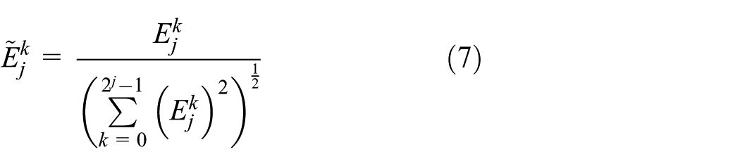
The algorithm of WPD can be summarized as follows. Let the coefficient of the nth frequency band of the jth level be x_j,_n(k). The signal of the nth frequency band of the jth level is further decomposed into the 2nth and (2n + 1)th frequency bands in the (j + 1)th level. The coefficients of the 2nth and (2n+1)th frequency bands, that is, x_j_+1,2n(k) and x_j_+1,2n+1(k), are calculated by equation (4). The decomposition process creates a full binary tree. The inverse process is the reconstruction process, in which the coefficient x_j,_n(k) can be reconstructed from x_j_+1,2n(k) and x_j_+1,2n+1(k), as given in equation (5)

{\begin{matrix} x_{j + 1, 2 n} (m) = \sum_{k \in Z} h_{k - 2 m} x_{j, n} (k) \\ x_{j + 1, 2 n + 1} (m) = \sum_{k \in Z} g_{k - 2 m} x_{j, n} (k) \end{matrix}

(4)

x_{j, n} (m) = \sum_{k \in Z} h_{m - 2 k} x_{j + 1, 2 n} (k) + \sum_{k \in Z} g_{m - 2 k} x_{j + 1, 2 n + 1} (k)

(5)

Equations (4) and (5) are the processes of wavelet packet decomposition and reconstruction, respectively.

WPD-based energy extraction algorithm

WPD decomposes the original signals orthogonally into 2^j frequency bands in the jth layer, where j can be any positive integer theoretically. Therefore, the signals in different frequency bands are orthogonal and independent of each other and satisfy the law of conservation of energy. The energy distribution of the frequency bands contains abundant non-stationary and nonlinear vibration information and is thus extracted here as the feature that identifies the different fault modes. The process of constructing the feature vector is detailed as follows:

Step 1. Perform j-level WPD on the acquired vibration signal and compute 2^j coefficients of each frequency band of the jth level using equation (4);

Step 2. Reconstruct the coefficients of each frequency band using equation (5). The 2^j reconstructed time-domain signals of the jth level are denoted as ${x_{k} | k = 0, 1, \dots, 2^{j} - 1}$ . Note that x_k is a vector of length N, that is, $x_{k} = [x_{k, 1}, x_{k, 2}, \dots, x_{k, N}]$ , where N is the length of the original signal;

Step 3. Compute the energy of each frequency band of the jth level, as given in equation (6), where x_k,_i is the element of the vector x_k

E_{j}^{k} = \sum_{i = 1}^{N} {(x_{k, i})}^{2}

(6)

Step 4. Construct the feature vector. Since the energy distribution of the frequency bands varies as the lubrication condition of linear rolling guides changes, the energy distribution is constructed as the feature vector to characterize the lubrication modes, denoted as $FV = [E_{j}^{0}, E_{j}^{1}, \dots, E_{j}^{2^{j} - 1}]$ . The energy is normalized, as given in equation (7)

{\tilde{E}}_{j}^{k} = \frac{E_{j}^{k}}{{(\sum_{k = 0}^{2^{j} - 1} {(E_{j}^{k})}^{2})}^{\frac{1}{2}}}

(7)

Case study

In this section, the lubrication–vibration experiments are carried out. The fault modes in this article refer to the three lubrication conditions (or patterns) labeled as “Poor,”“Medium,” and “Good.” The condition “Poor” is simulated through removing the original lubricant from the linear rolling guide. Poor lubrication will increase the friction and exacerbate the wear, causing abnormal vibration, accelerating the damage of the machine tool, and affecting the quality of machining. The condition “Medium” is simulated by lubricating the linear rolling guide with oil (lubricant type MOBILVG68). This condition is better than “Poor” but is still not very satisfactory. The condition “Good” is simulated by lubricating the linear rolling guide with grease (lubricant type Shell Gadus S2 V1003). This is the best case in the real working condition, which can reduce friction and noise while increasing the life and reliability of the linear guide. Vibration signals corresponding to the three lubrication conditions during the operation of the linear rolling guide are acquired. The raw signals are further analyzed by WPD. In the experiments, the ball linear rolling guide is used, the schematic of which is illustrated in Figure 2. Two linear rolling guides labeled as HJG-DA45 and GGB45 from different companies are used in the lubrication–vibration experiments, as shown in Figure 3.

Figure 2.

Schematic of ball linear rolling guide.

Figure 3.

Two linear rolling guides used in the experiments:(a) HJG-DA45 and (b) GGB45.

The linear rolling guide is installed on a reliability test bench that is independently developed in our laboratory, as shown in Figure 4. The drive system of the test bench drives the carriage of the linear rolling guide sliding along the rail. The accelerometer is affixed on the top surface of the carriage. The accelerometer is connected to the Prosig P8020 data acquisition system, which is connected to a computer through cables. The software named “Acquisition V4” is employed to acquire the vibration signals. The test bench and the data acquisition system are shown in Figure 5.

Figure 4.

Reliability test bench used in the experiments.

Figure 5.

Data acquisition system.

In all the three lubrication conditions of the experiments, the speed of the carriage is set to be 50 mm/s and the sampling frequency is 5 kHz. Signals of 8 s duration are acquired in each condition. The HJG-DA45 and GGB45 linear guides are tested sequentially. The procedure of the test is detailed as follows:

Step 1. Remove the carriage from the guide rail and clean the original lubricant on the return unit, rolling ball, and guide raceway with kerosene;

Step 2. Inject the lubricating oil MOBILVG68 into the carriage from the grease nipple;

Step 3. Run the carriage for 5 min at a speed of 50 mm/s in order to make the lubrication fully uniform;

Step 4. Set the sampling frequency of the data acquisition system to be 5 kHz. Acquire 8-s vibration signals after full lubrication;

Step 5. Repeat the above steps. It should be noted that in the case of “Good” lubrication, replace the lubricant with Shell Gadus S2 V1003 in Step 2, and in the case of “Poor” lubrication, skip Step 2.

Results and discussion

In this section, the feature extraction approach using WPD detailed in section “Feature extraction using WPD” is applied on the raw signals of the linear rolling guides acquired in section “Case study.” The energy distribution after a four-level WPD is extracted as the “feature.” The differences of the features from the three lubrication conditions are analyzed in section “Energy distribution of different lubrication patterns.” The relation between “features” and their corresponding lubrication conditions are revealed. In addition, to verify the effectiveness of the feature, a typical feedforward BP neural network is employed as the classifier. The results are reported in section “Fault diagnosis using neural network with energy distribution as input.”

Energy distribution of different lubrication patterns

The time-domain vibration signals of the three conditions of the linear guide GGB45 are illustrated in Figure 6. We see that the vibration amplitude in the case of “Good” lubrication is slightly smaller than those in the other two cases. However, it is still difficult to visually distinguish the three conditions based on their raw signals from the time domain. We transform the signal into the frequency domain using fast Fourier transform (FFT), as shown in the first column of Figure 7. The frequency range in which the first “peaks” appear is magnified and the corresponding results are presented in the second column. It can be seen that the differences among the three cases are not obvious and it is hard to see appropriate features to classify different cases. Therefore, the raw signals should be further analyzed in order to manifest the relation between the signal and the lubrication levels.

Figure 6.

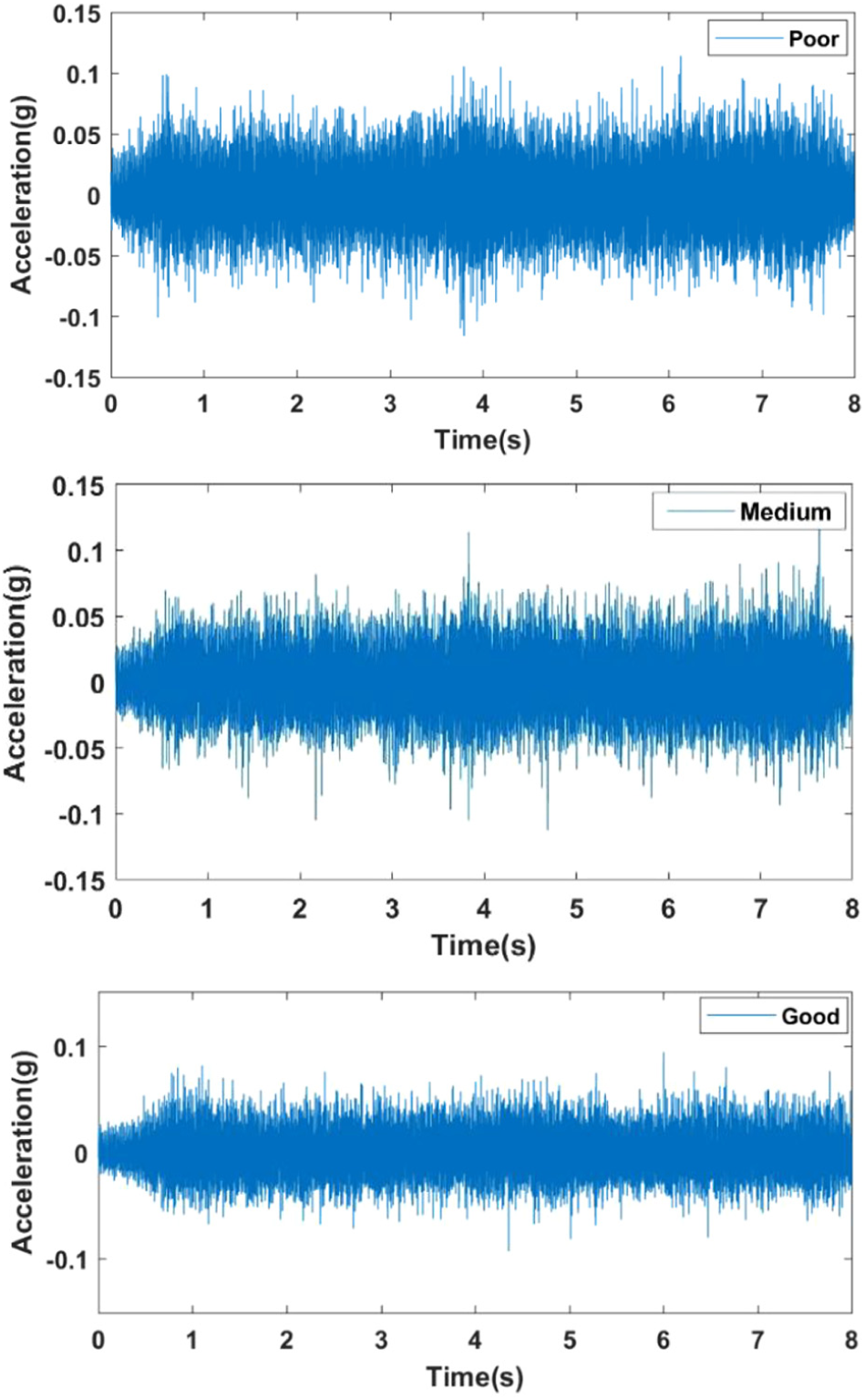
Raw vibration signals of the three lubrication conditions of GGB45.

Figure 7.

Frequency-domain signals of the three lubrication conditions of GGB45.

The WPD method detailed in section “Feature extraction using WPD” is employed. Daubechies 4 (db4) wavelet is selected as the basis function. A four-level decomposition is performed on the raw signals and 16 frequency sub-bands are obtained. The decomposition binary tree is shown in Figure 8. Note that according to the Nyquist sampling theorem the width of each frequency sub-band is 156.25 Hz. Therefore, the frequency bands of the 16 sub-bands are calculated as (n – 1) × 156.25 Hz ∼ n × 156.25 Hz, where n = 1, 2, …, 16, representing from the left to right the number of the sub-band in the last level of the binary tree. The 16 frequency sub-bands are further reconstructed using equation (5) to obtain 16 time-domain signals. The reconstructed signal of each packet in the last layer after a four-level decomposition of the linear rolling guide GGB45 is illustrated in Figure 9 as an example. Finally, the energy of each sub-band is calculated by equation (6) and normalized by equation (7). The energy distributions in the last layer of the linear rolling guides GGB45 and HJG-DA15 are shown in Figure 10.

Figure 8.

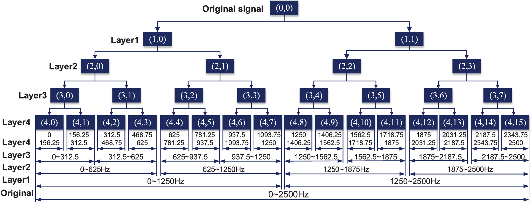
Binary tree of a four-level decompositon.

Figure 9.

Reconstructed signal of each packet of GGB45.

Figure 10.

Energy distribution under the three lubrication conditons: (a) type of linear rolling guide—GGB45 and (b) type of linear rolling guide—HJG-DA45.

The energy distributions in the three lubrication conditions of the linear rolling guides GGB45 and HJG-DA45 are shown in Figure 10. We see that in the first eight frequency sub-bands the energy of the vibration signal increases with the improvement of lubrication condition, while in the last eight frequency sub-bands this law is opposite, that is, the energy of the vibration signal decreases with improved lubrication. This can be interpreted as follows: the low-frequency vibration of the linear rolling guide is mainly caused by the oscillation of oil film. Therefore, in the first eight frequency sub-bands, the better the lubrication is, the larger the oscillation amplitude of the oil film, leading to larger signal energy. In contrast, the high-frequency vibration of the linear rolling guide is mostly due to friction. In the last eight frequency sub-bands, the better the lubrication is, the smaller the friction is, leading to smaller energy. After a four-level decomposition using WPD on the raw vibration signals acquired under the three lubrication conditions, the energy distributions of the vibration signals in the 16 frequency sub-bands follow a certain rule, which can be used as the feature vector to identify different lubrication conditions.

Fault diagnosis using neural network with energy distribution as input

In order to verify whether the energy distribution is an appropriate feature that can be used for fault diagnosis, we applied the feedforward BP neural network as the classifier to implement fault diagnosis. The neural network can be seen as a nonlinear mapping seeking to find a function that best maps a set of inputs to their correct outputs. It has been widely used to address various classification and regression problems. The BP neural network uses the BP method to calculate a gradient that is needed in the calculation of weights to be used in the network. The theory of BP neural network is not the main focus of this article and readers may refer to Sadeghi²⁵ for more details.

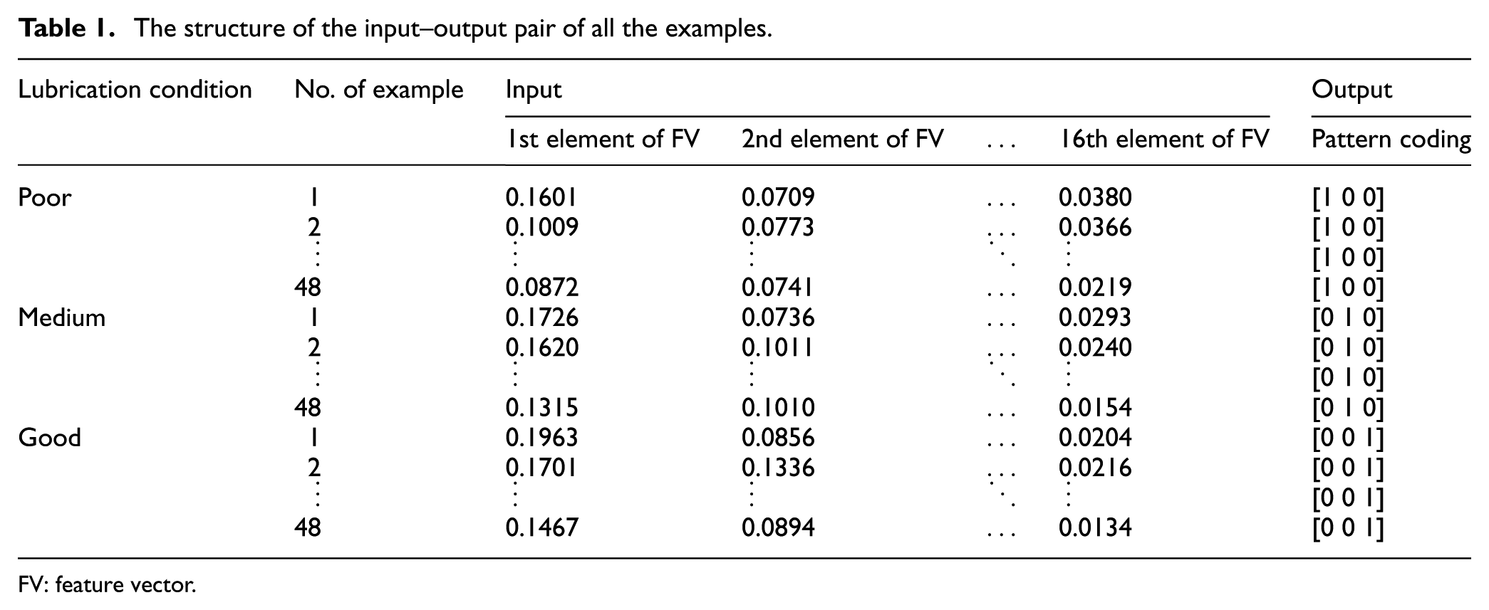
Reminder that in the experiment, for each lubrication condition, the sampling rate is 5 kHz and 8-s signals are acquired in one round. A 1-s segment of the signal (i.e. 5000 data points) is regarded as an example and hence in one round eight examples are acquired. We performed six rounds for each lubrication condition. Therefore, 48 examples are acquired for each condition and a total of 144 examples can be obtained. A four-level WPD followed by an extraction of energy distribution using the algorithm detailed in section “WPD-based energy extraction algorithm” is applied to each example. As a result, a feature vector with the length of 16 is extracted for each example. The feature will be used as the input of the BP neural network, while the output is one of the three lubrication patterns. For classification, the three patterns “Poor,”“Medium,” and “Good” are encoded as [1 0 0], [0 1 0], and [0 0 1], respectively. The structure of the input–output pair of all the examples is presented in Table 1.

Table 1.

The structure of the input–output pair of all the examples.

Lubrication condition	No. of example	Input				Output
Lubrication condition	No. of example	1st element of FV	2nd element of FV	…	16th element of FV	Pattern coding
Poor	1	0.1601	0.0709	…	0.0380	[1 0 0]
	2	0.1009	0.0773	…	0.0366	[1 0 0]
	⋮	⋮	⋮	⋱	⋮	[1 0 0]
	48	0.0872	0.0741	…	0.0219	[1 0 0]
Medium	1	0.1726	0.0736	…	0.0293	[0 1 0]
	2	0.1620	0.1011	…	0.0240	[0 1 0]
	⋮	⋮	⋮	⋱	⋮	[0 1 0]
	48	0.1315	0.1010	…	0.0154	[0 1 0]
Good	1	0.1963	0.0856	…	0.0204	[0 0 1]
	2	0.1701	0.1336	…	0.0216	[0 0 1]
	⋮	⋮	⋮	⋱	⋮	[0 0 1]
	48	0.1467	0.0894	…	0.0134	[0 0 1]

FV: feature vector.

A three-layer BP neural network is employed here. The numbers of neurons in the input layer and output layer are 16 and 3, which are equal to the length of the feature vector and to the length of the pattern coding, respectively. A hidden layer containing 10 neurons is adopted. The 144 examples are randomly divided into training set and testing set. We used 70% (100) for training and 30% (44) examples for testing. The learning rate of the BP algorithm is set to be 0.1. The classification results of the testing set are illustrated by a testing accuracy matrix as shown in Figure 11.

Figure 11.

Testing accuracy matrix.

In the matrix, the rows correspond to the output pattern of the network and the columns correspond to the target. The diagonal cells correspond to the examples that are correctly classified (the green cells), that is, the output is equal to the target, while the off-diagonal cells correspond to the incorrectly classified examples (the red cells). In each cell, both the number of example and the percentage of the total number of examples are shown. We can see that in the testing set there are 12 examples of “Poor,” 15 examples of “Medium,” and 17 examples of “Good,” corresponding to 27.27%, 34.09% (which is equal to 31.82% + 2.27%), and 38.64% of the total number of testing examples, respectively. The last column in the matrix shows the percentages of examples predicted to belong to each pattern that are correctly classified. This percentage is called the positive value. For example, there are 18 examples that are classified by the network into the pattern “Good,” while in fact 17 out of these 18 are correctly classified and one example that should actually belong to “Medium” is incorrectly classified as “Good.” The positive value is hence 94.4%. The row at the bottom of the matrix shows the percentages of all the examples belonging to each class that are correctly classified. For example, there are 15 examples of “Medium” in the testing set. Out of these 15 examples, 14 are correctly classified and 1 is incorrectly classified as “Good.” The percentage is thus 93.3%. The value in the bottom right corner is the overall correct rate of the network, which is equal to the number of correctly classified examples divided by the total number of examples, which in this case is 97.7%.

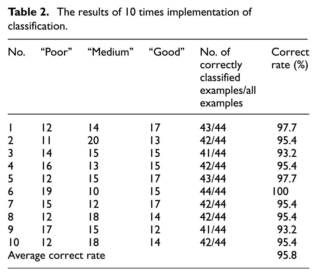
Since each of the 144 examples is randomly being picked as the training or testing example, the training set and the testing set may change every time when implementing the classification. In order to verify the robustness of our method, we implement the classification 10 times. In each implementation, the number of “Poor,”“Medium,” and “Good” patterns, the number of correctly classified examples over the number of all examples, and the correct rate are recorded. The results are presented in Table 2, from which we see that the average correct rate of the network is 95.8%. This indicated that the energy distribution can be used as an appropriate feature for fault diagnosis of linear rolling guide.

Table 2.

The results of 10 times implementation of classification.

No.	“Poor”	“Medium”	“Good”	No. ofcorrectlyclassifiedexamples/allexamples	Correctrate (%)
1	12	14	17	43/44	97.7
2	11	20	13	42/44	95.4
3	14	15	15	41/44	93.2
4	16	13	15	42/44	95.4
5	12	15	17	43/44	97.7
6	19	10	15	44/44	100
7	15	12	17	42/44	95.4
8	12	18	14	42/44	95.4
9	17	15	12	41/44	93.2
10	12	18	14	42/44	95.4
Average correct rate					95.8

Conclusion

This article demonstrates the relation between different lubrication conditions of linear rolling guide and their corresponding vibration signals through lubrication–vibration experiments. The three lubrication conditions labeled as “Poor,”“Medium,” and “Good” are simulated by removing the original lubricant, lubricating using oil, and lubricating using grease, respectively, representing different lubrications in the actual working conditions. A data acquisition system was set up to acquire the vibration signals corresponding to the three conditions during the operation of the linear rolling guide.

WPD was employed to extract energy distribution as a “feature” from the raw signal. Two linear rolling guides manufactured by different companies were used in the experiments. The results showed that for both linear rolling guides the relation between “features” and their corresponding lubrication conditions follows certain rules. Specifically, in low-frequency sub-bands of the vibration signals, energy increased when the lubrication improved, while in the high-frequency sub-bands energy decreased with improved lubrication. This finding shows that the lubrication conditions can be characterized by “energy” hidden in the vibration signals, indicating that energy can be used as a feature for health diagnosis of linear rolling guide.

In addition, to verify the effectiveness of the feature, 48 segments of signals of each lubrication pattern were acquired, forming a total number of 144 segments. The energy distribution of each segment was extracted as one example of feature vector. We randomly chose 70% of the 144 examples for training and the rest 30% for testing. A three-layer feedforward BP network was used as the classifier. The results showed that the average classification accuracy of the network that uses energy distribution as the input was more than 95%. This indicated that the energy distribution can be used as an appropriate feature for fault diagnosis of linear rolling guide.

Footnotes

Handling Editor: Zengtao Chen

Declaration of conflicting interests

The author(s) declared no potential conflicts of interest with respect to the research, authorship, and/or publication of this article.

Funding

The author(s) disclosed receipt of the following financial support for the research, authorship, and/or publication of this article: This work was supported by the National Science and Technology Major Project of China (grant no. 2017ZX04011001).

ORCID iD

Yiwei Wang

References

Zou

Wang

BL.

Investigation of the contact stiffness variation of linear rolling guides due to the effects of friction and wear during operation. Tribol Int 2015; 92: 472–484.

Hung

JP.

Load effect on the vibration characteristics of a stage with rolling guides. J Mech Sci Technol 2009; 23: 89–99.

Tao

Zhong

Feng

et al . Model for wear prediction of roller linear guides. Wear 2013; 305: 260–266.

Wang

Gogu

Binaud

et al . A cost driven predictive maintenance policy for structural airframe maintenance. Chin J Aeronaut 2017; 30: 1242–1257.

Wang

Gogu

Binaud

et al . Predictive airframe maintenance strategies using model-based prognostics. Proc IMechE, Part O: J Risk and Reliability. Epub ahead of print 1March2018. DOI: 10.1177/1748006X18757084

Zhang

Mansaf

et al . Gear wear monitoring by modulation signal bispectrum based on motor current signal analysis. Mech Syst Signal Pr 2017; 94: 202–213.

Glowacz

et al . Early fault diagnosis of bearing and stator faults of the single-phase induction motor using acoustic signals. Measurement 2018; 113: 1–9.

Park

Kim

Choi

JH.

Gear fault diagnosis using transmission error and ensemble empirical mode decomposition. Mech Syst Signal Pr 2018; 108: 262–275.

Sharma

Upadhyay

Kankar

et al . Nonlinear dynamic investigations on rolling element bearings: a review. Adv Mech Eng 2018; 10: 764148.

10.

Saucedo-Dorantes

Delgado-Prieto

Ortega-Redondo

JAO

et al . Multiple-fault detection methodology based on vibration and current analysis applied to bearings in induction motors and gearboxes on the kinematic chain. Shock Vib 2016; 2016: 1–13.

11.

Sawalhi

Wang

Becker

Vibration signal processing for spall size estimation in rolling element bearings using autoregressive inverse filtration combined with bearing signal synchronous averaging. Adv Mech Eng 2017; 9: 703007.

12.

Guo

Gao

Lei

. Methodology for ball screw support bearing fault analysis with screw nut vibration signal. In: Proceedings of the 2015 prognostics and system health management conference (PHM), Beijing, China, 21–23 October 2015, pp.1–6. New York: IEEE.

13.

Baraldi

Di Maio

et al . A systematic semi-supervised self-adaptable fault diagnostics approach in an evolving environment. Mech Syst Signal Pr 2017; 88: 413–427.

14.

Lei

Jia

Lin

et al . An intelligent fault diagnosis method using unsupervised feature learning towards mechanical big data. IEEE T Ind Electron 2016; 63: 3137–3147.

15.

Dhamande

Chaudhari

MB.

Compound gear-bearing fault feature extraction using statistical features based on time-frequency method. Measurement 2018; 125: 63–77.

16.

Deep learning based approach for bearing fault diagnosis. IEEE T Ind Appl 2017; 53: 3057–3065.

17.

Zhong

Wong

Yang

ZX.

Fault diagnosis of rotating machinery based on multiple probabilistic classifiers. Mech Syst Signal Pr 2018; 108: 99–114.

18.

Mao

Yan

et al . Online sequential prediction of bearings imbalanced fault diagnosis by extreme learning machine. Mech Syst Signal Pr 2017; 83: 450–473.

19.

Jia

Lei

Guo

et al . A neural network constructed by deep learning technique and its application to intelligent fault diagnosis of machines. Neurocomputing 2018; 272: 619–628.

20.

García Plaza

Núñez López

. Application of the wavelet packet transform to vibration signals for surface roughness monitoring in CNC turning operations. Mech Syst Signal Pr 2018; 98: 902–919.

21.

Wang

Zhu

et al . Design of online monitoring and fault diagnosis system for belt conveyors based on wavelet packet decomposition and support vector machine. Adv Mech Eng 2013; 5: 797183.

22.

Wang

Fault diagnosis method based on wavelet packet-energy entropy and fuzzy kernel extreme learning machine. Adv Mech Eng 2018; 10: 751446.

23.

Bianchi

Mayrhofer

Gröschl

et al . Wavelet packet transform for detection of single events in acoustic emission signals. Mech Syst Signal Pr 2015; 64–65: 441–451.

24.

Fei

SW.

Fault diagnosis of bearing based on relevance vector machine classifier with improved binary bat algorithm for feature selection and parameter optimization. Adv Mech Eng 2017; 9: 685294.

25.

Sadeghi

BHM

. A BP-neural network predictor model for plastic injection molding process. J Mater Process Technol 2000; 103: 411–416.

Feature extraction for fault diagnosis based on wavelet packet decomposition: An application on linear rolling guide

Abstract

Keywords

Introduction

Feature extraction using WPD

Decomposition and reconstruction of wavelet packet

WPD-based energy extraction algorithm

Case study

Results and discussion

Energy distribution of different lubrication patterns

Fault diagnosis using neural network with energy distribution as input

Conclusion

Footnotes

Declaration of conflicting interests

Funding

ORCID iD

References