
Abstract
It is generally observed that special channels exit in many key components of machine, such as non-linear tube, applied in military or civil industries. Its surface finish is a crucial factor in the whole performance of machine. In military and civil fields, many key parts have special passages, such as non-linear tube. The surface quality of non-linear tube usually decides the general using property of the whole equipment. The abrasive flow machining technology can effectively improve the surface quality of non-linear tube parts and promote the using property of the whole equipment. The technology of solid-liquid two-phase abrasive flow machining can obtain higher enhancement in surface quality. To investigate the processing technology of abrasive flow machining for non-linear tube–injection nozzle, we performed a full factorial experiment modifying critical process parameters such as particle density, particle size, and abrasive viscosity during the machining. The study investigated the relationship among abrasive particle physical property, surface quality of non-linear tube, and the optimal parameters. At the same time, we deduced the regression equation which takes the abrasive particle physical property as the key factor. Through full factorial experimental study, it is found that under the experimental conditions of this article, abrasive flow polishing process serves best when the abrasive concentration is 10% and the particle size is 6 μm. Moreover, the verification experiment of the non-linear nozzle is carried out. The average value of the experimental data is located in the prediction interval, which confirmed the accuracy of the whole factor test. The experimental results can provide technical support for further research of abrasive flow machining theory. The research results in this article have profound theoretical significance and practical value for improving the machining efficiency of non-linear parts and obtaining high-quality-surface passages. The study data possess important theory significance and practical value for improving the processing efficiency for non-linear tube and obtaining a high-quality surface channel. The experimental results can provide technology support for further study on abrasive flow machining theory.
Keywords
Introduction
It is generally observed that high-performance channels exit in many key component of the military and civil industries, ranging from some critical component in oil feeding system to intake and exhaust system of infantry fighting vehicle, from aircraft engine air-cool channel to special channel, and cross inner hole in satellite attitude control system, as well as many complex molds. 1 Surface quality of critical component determines the whole performance, so people urgently need to enhance the surface quality to reduce wear, obtain better fitting accuracy, higher fatigue strength and corrosion resistance, and other performance. Because of this, abrasive flow machining (AFM) technology comes true into being. AFM technology plays an effective role in ultra-precision machining for complex component inner channel surface.2,3
Abrasive flow polishing is a latest developed processing method in recent decades, using liquid (oil) as the carrier and hard particles (silicon carbide as general) as cutting tools which flow through the surface of a workpiece under a certain value of speed or pressure, so as to achieve precision machining. The distinctive advantage of the technology is that it is barely subject to limitations of components’ shape or size, more evident for parts with complex channels. A schematic diagram of abrasive flow polishing is shown in Figure 1.

Polishing sketch of abrasive flow machining.
Many researchers have put forward their research report. RK Jain and colleagues4,5 carried out the test study of material removal rate and surface roughness, and the result is that the principal grinding ways in AFM is scratch function of abrasive particle. RS Walia et al.6,7 studied the effect of centrifugal force for AFM process and drew the conclusion that the X-ray diffraction (XRD) analysis and optical micro-photographs of test specimens have shown that centrifugal force assisted abrasive flow machining (CFAAFM) process did not affect the surface micro-layer during processing under any of the conditions used for this study and the increase in surface micro-hardness and residual compress stress of workpiece with the increase in rotational speed of centrifugal force generating (CFG) rod can be attributed to the machining hardening of the workpiece surface that might occur due to “throw” of abrasive particles upon specimen surface. MR Sankar et al.8,9 investigated the processing property of rotary AFM and the relationship of workpiece velocity of rotation, number of processing, extrusion stress, percentage of medium, and surface roughness. KK Kar et al. 10 studied the temperature of inflow, shear rate, and frequency on rheological behavior and percentage of abrasive flow medium. MR Sankar et al. 11 investigated the influence of abrasive flow rotary machining on workpiece surface topography. H Zarepour and SH Yeo 12 took mono-abrasive as research object and studied material removal mode in ultrasound assistant micro-machining. Y-Q Tan et al. 13 numerically simulated the flow pattern of abrasive flow during AFM. L Fang et al. 14 studied the relationship of temperature and viscosity and performed relative simulation. S-M Ji and colleagues.15,16 presented a new mold structural surface no-tool precision finish machining method based on soft abrasive flow. K Zhang et al. 17 analyzed the internal factor in AFM by building mechanical model. MR Sankar et al. 18 discussed rotational abrasive flow finishing process, preliminary experiments are conducted on Al alloy and Al alloy/SiC metal matrix composites at different extrusion pressures, and medium compositions are employed for finding optimum conditions of the same for higher change in roughness; they proposed the mechanism of material removal of matrix and reinforcement in metal matrix composites using rotational abrasive flow finishing. S Rajesha et al. 19 have studied the abrasive flow characteristics of polymer abrasive. J Kenda et al. 20 use the abrasive flow technology to plastic gear-matrix polishing and discuss the effect of processing time on the processing quality, abrasive of which is still polymer abrasive. AC Wang and SH Weng 21 machine the workpiece produced by wire electrical discharge, using polymer abrasive gels, ending up with the surface roughness decreasing from 1.8 to 0.28 µm. HS Mali and A Manna 22 polish SiCp-MMC workpiece by abrasive flow technology to discuss the influence of abrasive mesh size, number of cycles, extrusion pressure, percentage of abrasive concentration, and media viscosity grade on finishing quality. VK Gorana et al. 23 have discussed the influence of parameters such as extrusion pressure and percent abrasive concentration on finishing result.
However, most previous experimental studies and theories were based on some special conditions, which had limited effects on universal guiding significance of AFM technology. The current research of AFM is mostly done by AFM with polymer abrasive. In this article, a full factorial process test is carried out on a non-linear tube nozzle with self-developed solid-liquid two-phase abrasive flow abrasive. The solid-liquid abrasive flow abrasive developed by ourselves in this article can make precise polishing of small hole parts, and the polymer abrasive cannot realize the precision polishing of small holes because of its high viscosity. The use of the same will cause damage to the workpiece, so that it cannot achieve effective polishing. In this article, a self-developed abrasive flow abrasive is used to study the non-linear tube and injection nozzle, and the viscosity grade parameters in the grinding and polishing process are considered. It is of great practical significance for the development of the precision polishing technology for solid and liquid two-phase abrasive flow. It can provide important theoretical and technical support for the practical grinding and polishing of abrasive flow.
Design scheme of whole factorial experiment
Whole factorial experiment, this very practical, concise methodology, can obtain many useful data by statistical analysis. Therefore, it is widely used by engineers. Whole factorial experiment design is a way combining all levels of all factors and scheduling one test at least for every combination. The advantage of whole factorial experiment lies in analysis of main effect and interaction effect for whole factors. When the number of study factors is small and interaction needs to be analyzed, whole factorial experiment design is the best option. Analysis process of whole factorial experiment is shown in Figure 2.
Step one: fitting model

Flow chart of whole factorial experiment design.
Fitting the selected model is a mathematical model selected according to the purpose of the experiment. This mathematical model usually includes all the factors contained in the test process and the two-order interaction between factors. By analyzing the selected models, we can conclude which factors are effective and which ones are not. When choosing the next fitting model, we only consider the significant items. The key parameters are as follows:
(a) The total effect in the ANOVA table.
The hypothesis tested in this item is:
If the p value of the corresponding regression term is less than 0.05, it indicates that the original hypothesis should be rejected, that is, the model can be judged to be effective on the whole; If the p value of the corresponding regression term is greater than 0.05, on the other hand, it shows that the original hypothesis cannot be rejected, that is to say, the model can be found generally invalid.
(b) Unfitting phenomena in the ANOVA table.
The hypothesis tested in this item is:
In the results of analysis of variance (ANOVA), if the corresponding p value of the misplaced item is greater than 0.05, it can be concluded that there is no misfit phenomenon in the model; Otherwise, some critical items may be missed during the model selection and reestablishing the model should be considered.
(c) The bending terms in the ANOVA table.
The hypothesis tested in this item is:
In the results of ANOVA, if the p value corresponding to the bending term is greater than 0.05, it shows that the model does not have a bending phenomenon; on the other hand, the data are curved, and the square term should be reclassified into the model.
(d) Correlation coefficient of fitting total effect:
By comparing the proximity of R2 (adj) to R2, it is possible to judge whether the model is improved or not; the closer the two, the better the model. In the analysis process, the original model chosen usually contains all factors, namely “whole model.” Then, insignificant factors are crossed out, and modified model is obtained. If R2 (adj) is closer to R2 in the modified model than that of whole model, it can be said that the model has been improved.
(e) Pareto effect diagram and normal effect plot.
It is very intuitive to use the Pareto effect diagram to determine the significance of the factor effect, but it has an obvious disadvantage: at the beginning of t-examination of each effect, the value of
Order the effect of each factor and mark it in the normal probability graph to form a normal effect diagram. It is basically considered that only a few factors are significant effect factors, which is called effect sparsity principle. Therefore, the effect of the point group is located in the middle of the fitted line, with the line as the observation criteria to determine which ones are significant effect factor. Principle is that factor far from the linear factor can be considered as an effective one and close to the line an effect is not significant.
Through the analysis of the above parameters, the first step of “fitting the selected model” is completed.
2. Second step: residual diagnosis
Carefully examine the four graphics automatically output by a computer:
Observe the scatter plot of the residual on the observed values and check out whether the scattered points are randomly distributed over the transverse axis.
Observe the scatter plot of the residuals on the fitting value of the response variable and see if the residual difference is equal variance distribution.
Observe the normality test chart of the residuals to determine whether the distribution of residual is in accordance with the normal distribution.
Observe the scatter plot of the residuals on the independent variable, mainly to see if there is a bending trend.
If the four graphs of the residual diagnosis are all normal, the model is normal.
3. The third step is to estimate whether the model needs to be improved or not.
Based on the results of the first and second steps, we can determine through the two aspects, numerical analysis and residual diagram, whether the model needs to be improved and how. In addition, based on the saliency of each effect, after deleting the non-significant items in the model, we found that there was a need for modification in the model, and returned to the original first step, and finally established the model.
4. The fourth step is to analyze the interpretation model.
(a) From the main effect diagram and interaction effect diagram, we further identify whether the selected factors and interaction items are truly significant, and whether the main effect and interaction effect of those factors are really not significant, thereby confirm the selected model more specifically and intuitively.
(b) Find out the best value in the whole experiment range. In the stage of factor design, the purpose of experimental design is to filter variables, but in fact, in the first step of Design of Experiments (DOE) analysis, we can already determine which variables are significant and which ones are not. We can get the optimal value based on these information.
5. The fifth step: determine whether the goal has been achieved.
It is mainly to compare the target value of the analysis and prediction with the original experimental target. If it is far from the target, a new round of experiments should be considered. If the target is basically reached, a test should be carried out to predict whether the effect is effective.
The whole factor test parameters of the abrasive flow processing must be selected first before the full factor test is carried out. It is found that the injection nozzle has the best processing quality when the abrasive flow processing time is 60 s, and the processing time selected in this article is 60 s. The material properties of the abrasive flow processing quality are tested by the self-configured abrasive flow polishing liquid. In the experiment, fuel nozzle is regarded as study object. Principal factors affecting the abrasive media performance are abrasive density, abrasive particle size, and abrasive viscosity. The aim of the experiment is that principal factors are how to affect the surface quality of nozzle channel during AFM. Based on theory and experiment analysis, appropriate values for the above parameters are set, as shown in Table 1.
Machining parameters and different values of fuel spray nozzle in AFM.
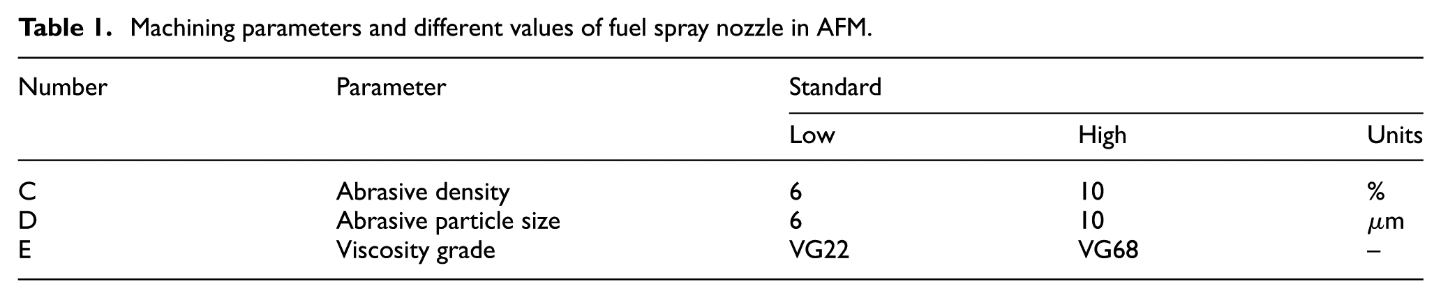
At first, Ra of nozzle hole channel was chosen as response variable and then a whole factorial experiment was conducted following Table 1. The numbers 22, 46, and 68 denote the viscosity grade. The viscosity grade (VG) of ISO to oil is divided according to its kinematic viscosity at 40°C. The viscosity grades 22, 46, and 68 are international standardization organizations ISO VG22, ISO VG46, and ISO VG68. On the basis of experimental study and test parameters in the literature, 2 the particle size of this study was selected as 6, 8, and 10 µm in this article. When the abrasive concentration reaches 12%, the abrasive flow processing is not smooth. Moreover, when the abrasive concentration is more than 15%, the abrasive will block the nozzle hole, the abrasive flow processing cannot continue, and the test will be forced to terminate. Therefore, the selection of abrasive concentration is 6%, 8%, and 10% in this experiment. Then, on the basis of experiment design table, 12 nozzle components were chosen to be examined. The experiment design and results are shown in Table 2.
AFM whole factorial experiment design table of fuel spray nozzle.

Results and discussion
Modeling
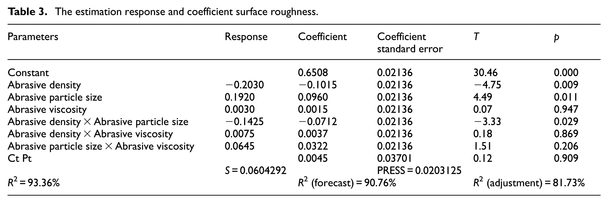
To begin with, abrasive density, abrasive particle size, abrasive viscosity, and their second-order interaction items (abrasive density × abrasive particle size, abrasive density × abrasive viscosity, abrasive density × abrasive viscosity) are taken as parameter settings of the model. Abrasive density × abrasive particle size represents the interaction between them, ditto for abrasive density × abrasive viscosity and abrasive density × abrasive viscosity. It is necessary that the analysis does not include the third-order interaction items (abrasive density × abrasive particle size × abrasive viscosity). By analyzing and calculating the selected model, the results are shown in Tables 3 and 4.
The estimation response and coefficient surface roughness.
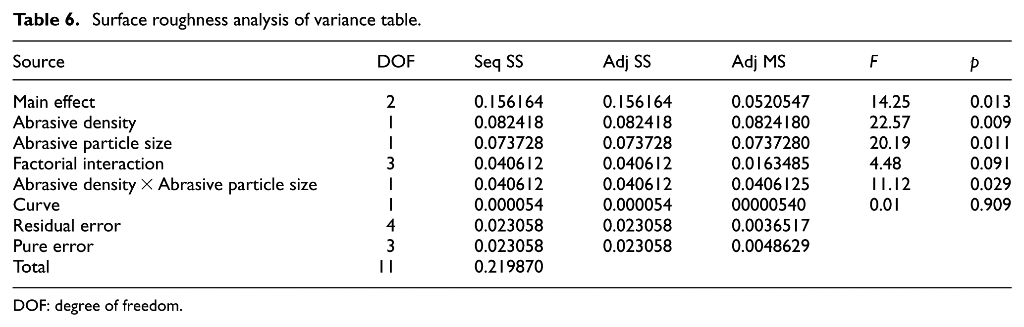
Surface roughness analysis of variance table.

DOF: degree of freedom; MS: mean square; SS: square sum of deviations.
Research aims at the value of p in variance analysis table and critical value of p is 0.05. When the value of main effect is below the critical value, it means the results of model are worth studying. When the value of bending item is greater than 0.05, it means the models do not have bending trend and when the value of lack of fit is greater than 0.05, it means the models do not have the property of lack of fit.
The surface roughness ANOVA table shows that the value of p in main effect item is 0.013 and less than 0.05; in bending items, the value of p is 0.909 and obviously greater than 0.05; the value of p in lack of fit item is 0.955 and clearly greater than 0.05. So we can draw a conclusion that total effect of the selected model is prominent and effective and the response variable indicates no bending trend or unfitting phenomenon.
From the surface roughness ANOVA table, the value of p for abrasive density is 0.009 and abrasive particle size is 0.011. Both of the values are less than 0.05. The value of p for abrasive viscosity is 0.947 and is much larger than 0.05. The value of p for the interaction of abrasive density and abrasive particle size is 0.029 and is less than 0.05; the value of p for the interaction of abrasive density and abrasive particle size is 0.869 and the interaction of abrasive particle size and abrasive viscosity is 0.206. Both of them are clearly greater than 0.05. Based on the above analysis, we can infer that abrasive density, abrasive particle size, and interaction of them are more effective for AFM of fuel spray nozzle. And then we verify further with Pareto plot and normal effect plot. Figure 3 is Pareto plot.

Standardized effect Pareto map.
In Figure 3, absolute values of significance level for factor C, factor D, and the interaction of them (CD) are greater than the given critical value and factor E and the interaction of them (CE, DE) is not. So factor C, factor D, and interaction of them (CD) is more effective. From Figure 4, we come out with the same decision, and it also confirms the same.

Normal plot of the standardized effects.
Residual error diagnosis
Calculate the output surface roughness residual plot and observe and analyze it. Surface roughness residual plot is shown in Figure 5.

Residual plot for surface roughness Ra.
In AND sequence graph, all the points in the horizontal axis show randomly irregular fluctuation, and there is no abnormal trend; in normality probability graph, the residuals remain equal; In AND fitted value graph, residuals comply with normal distribution; the residuals of surface roughness are within the normal range, indicating that the model is correct.
Model refinement
It is realized that not all of the independent variables are active effect terms through testing every term. In the three independent main variables, factor C (abrasive density) and factor D (abrasive particle size) are effective; factor E (abrasive viscosity) is not effective. In addition, among the three interactions of them, the CD is the only one effective factor and the other two (abrasive density × abrasive viscosity and abrasive particle size × abrasive viscosity) are not effective. So when refining the fitting model, we chose the effective one to reset the fitting model.
Fitting the selected model
Delete the ineffective terms, recalculate, and reanalyze. In the new selected model, the factors include factor C (abrasive density), factor D (abrasive particle size), and the interaction of them (abrasive density × abrasive particle size). In this model, we still apply the former method and procedure to analytical calculation, and analysis data obtained is shown in Tables 5 and 6.
The table of estimation response and coefficient surface roughness Ra.

Surface roughness analysis of variance table.
DOF: degree of freedom.
In ANOVA table, the values of main effect term and two-order interaction term are 0.001 and 0.010, and the values are less than 0.05, which demonstrates that the model is effective. The main effect term value is less than that (the value is 0.013) in old model. The value of p for bending error is 0.902 and is much greater than critical value (0.05), which indicates the model accords with linear hypothesis conditions. Collect the calculated data of R2, R2 (adj),and estimator of standard deviation in the two tables and make a table. Numerical comparison in pre- and post-improvement of model is shown in Table 7.
Results comparison of original model and modified model.

From Table 7, it can be seen that in the model improved, the value of R2 reduces to 0.8951 from 0.9336 and R2 (adj) rises from 0.8173 to 0.8352. The values are closer after deleting something from the old model, which means that the refinement of deleting the ineffective term is beneficial.
Residual error diagnosis
The residuals of the new model are diagnosed and the results are given in Figure 6. In AND sequence graph, all the points in the horizontal axis show randomly irregular fluctuation, and there is no abnormal trend; in normality probability graph, the residuals remain equal; in AND fitted value graph, residuals obey normal distribution; the residuals of surface roughness are within the normal range, indicating that the model is still solid.

Residual plot for surface roughness Ra.
Model refinement estimate
According to the above analysis, it is determined that the model does not need to be optimized further. According to the numerical results, the code regression equation can be acquired.
Based on the estimation effect and coefficient of surface roughness shown in Table 8, we can note down the code regression equation of surface roughness, which is formula (1)

The optimized table of estimation response and coefficient surface roughness Ra.

In formula (1), the coefficients come from the surface roughness estimation effect and coefficient table and 0.6508, −0.1015, and −0.0712 are, respectively, constant and corresponding coefficients of C (abrasive density), D (abrasive particle size), and CD (abrasive density × abrasive particle size). The number 8 of
Based on the regression equation, we can calculate the surface roughness with different abrasive densities and different particle sizes in this experiment condition.
Analyzing model
Perform detailed analysis and explanation through graphic information for obtained regression model. Figure 7 is surface roughness main effect plot.

Main effect plot for surface roughness Ra.
We can see from Figure 7 that the effect of factor C and factor D for response variable (surface roughness Ra) is significant, while the effect of factor E (abrasive viscosity) is not. The figure shows that in order to make the value of the surface roughness Ra smaller, the abrasive concentration should be as large as possible and the particle size as small as possible.
Figure 8 is the second-order interaction effect of three factors (abrasive density, abrasive particle size, and abrasive density) plot. The effect of interaction of abrasive density and abrasive particle size for response variable (surface roughness Ra) is significant (two lines are quite unparallel). And effect of the other interaction is not significant (two lines are quite parallel).

Interaction plot surface roughness Ra.
The response variable is surface roughness, which is a kind of “longing minimum” model optimization. In optimal target setting, our goal is obtaining minimum. So we only fill in “upper” and “goal” grids and the lower is blank. We set upper = 0.8 µm and goal = 0.4 µm. Then we can calculate the minimum of the surface roughness. The results are shown in Figure 9.

Output results plot of the response variables optimizer.
Usually we translate the question of optimized response available Y into a question about satisfaction of solving desirability function to reach maximum.
When the factor C is 10% and the factor D is 6 μm, the value of surface roughness will reach average minimum of 0.5345 μm. The output is given by d. The value of d means desirability function. When the results are closer to the setting goal, the value of d is closer to 1. The result of d is 0.68875 in this experiment, and it follows that the ideal minimum is 4 μm. The value of d will be different as the various settings of minimum.
Verification test
The calculation of the predictive value and the prediction interval
Our primary task is to calculate that to what kind of scope every experiment result will belong. If average of m times test results belong to the designed scope, it means the model is correct and predicted results are credible.
Confirmation prescription of prediction interval is successively filling the value of main effect into the factor item so that we can obtain predicted value and prediction interval (Table 9).
Prediction value and interval of regression analysis.
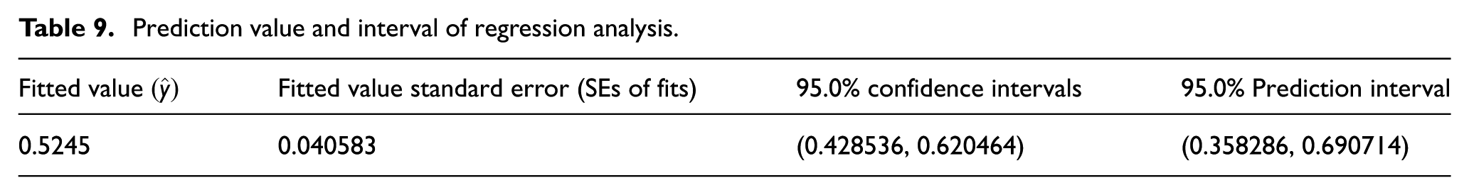
The 95% confidence interval refers to the confidence interval for discrete points on the regression equation. It means that with the current set of the independent variable running at an infinite number of times, results will be locked within a 95% confidence range of the theoretical mean value.
95% confidence interval is for one verification test. It refers to the variation range of the response variable at a test in accordance with the optimum level, which can be used for verification test.
95% confidence interval and 95% prediction interval calculated by regression analysis is for countless times and one time verification tests. If we want to calculate 95% confidence interval of m times (e.g. m = 3 or m = 5), we have to compile macro-instruction or directly use hand computation. The computational formula of 95% confidence interval with average of m times observed values is given by
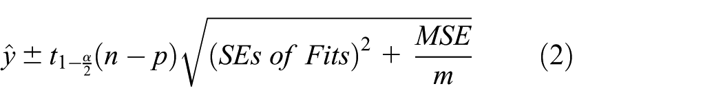
where
The number of verification test is usually greater than or equal to three times and we perform four times verification tests in this experiment. And in formula (3), n = 12, p = 3, m = 4, “SEs of Fits” = 0.040583, and MSE = 0.0032940.
Formula of variable radius is as follows
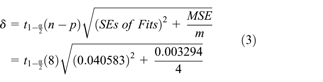

Variable radius δ = 0.1146.
So the 95% confidence interval of average for the four verification tests is

It means that the average of results of four verification tests is in this scope (0.4099, 0.6391). It argues that the model is right and the predicted results are believable. Otherwise, the model is fault and the predicted results are untrustworthy.
Test verification
Through full factor analysis, it is found that the surface roughness gets minimum when the abrasive concentration is 10% and the particle size is 6 μm. Choose the nozzle as an object of study, which has large hole diameter of 4 mm and small hole diameter of 0.16 mm. Four abrasive flow polishing experiments were carried out to verify the accuracy of the conclusion of the whole factor test. The four nozzles were labeled as sample 01#, sample 02#, sample 03#, and sample 04#. The body diagram of the fuel injector is shown in Figure 10. After polishing, the surface of the nozzle was detected by scanning electron microscope as shown in Figure 11.
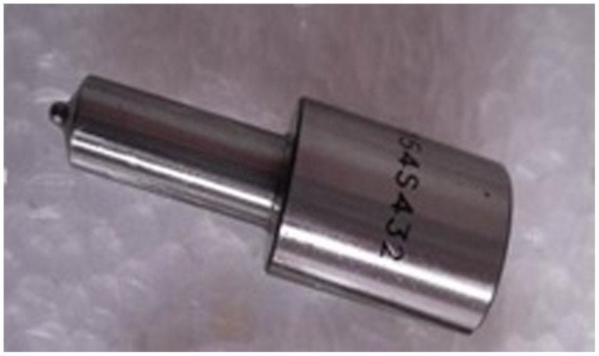
The physical picture of the nozzle for the test.

Contrast of surface morphology before and after polishing of injector nozzle: (a) original script, (b) Sample 01#,(c) Sample 02#, (d) Sample 03#, and (e) Sample 04#.
Figure 11(a) is the original surface morphology of the injection nozzle. Figure 11(b)–(e) shows sample 01#, sample 02#, sample 03#, and sample 04# after abrasive flow. Figure 12(a) is the original surface roughness diagram of the nozzle workpiece. From Figure 11, we can see that the surface morphology of the nozzle before and after polishing differs a lot. The surface of the nozzle is rough and uneven before abrasive flow polishing, and the surface tends to be smooth after abrasive flow polishing. In order to get the change of surface quality, the surface roughness of the nozzle is detected by grating surface roughness measuring instrument. The three-dimensional scanning map is shown in Figure 12.

Three-dimensional scanning of the injection nozzle before and after polishing: (a) original script, (b) Sample 01#, (c) Sample 02#, (d) Sample 03#, and (e) Sample 04#.
Figure 12(b)–(e) shows sample 01#, sample 02#, sample 03#, and sample 04# through the abrasive flow surface roughness after the surface roughness. From Figure 12, we can see that the surface roughness Ra before abrasive flow polishing was 1.03 μm, and the surface roughness Ra of the nozzle after abrasive flow polishing was, respectively, 0.45473, 0.56335, 0.55388, and 0.49189 μm, and the average surface roughness was Ra 0.51596 μm. The surface roughness of the nozzle is obviously reduced after polishing by the abrasive flow, and the surface quality of the nozzle is substantially improved. The obtained surface roughness values are within the prediction interval, indicating that the prediction results are credible and the model is effective.
Conclusion
Using the self-developed abrasive flow medium, nozzle is taken as the research object to carry out the whole factorial experiment. In the whole factorial experiment, the abrasive density, abrasive particle size, and abrasive viscosity are taken as main factors to explore in depth the effect of abrasive medium physical property on non-linear tube surface with AFM and optimum parameter combination was obtained. Through full factorial experimental study, it is found that under the experimental conditions of this article, abrasive flow polishing process serves best when the abrasive concentration is 10% and the particle size is 6 μm. On the basis of this parameter, the test is carried out, and the test data are consistent with the prediction interval, which confirms the validity of the whole factor test. AFM mathematical model is perfected by collecting, organizing, and analyzing experiment data and explored the inherent law of experiment data. And then a regression equation is deduced based on abrasive physical property. The regression equation can provide fundamental basis for quantitative control technology of AFM processing quality.
Footnotes
Handling Editor: Wen-Hsiang Hsieh
Declaration of conflicting interests
The author(s) declared no potential conflicts of interest with respect to the research, authorship, and/or publication of this article.
Funding
The author(s) disclosed receipt of the following financial support for the research, authorship, and/or publication of this article: The authors would like to thank the National Natural Science Foundation of China (No. NSFC 51206011) and Jilin Province Science and Technology Development Program (Nos 20160101270JC and 20170204064GX).