
Abstract
Today, short- and long-term structural health monitoring of bridge infrastructures and their safe, reliable and cost-effective maintenance have received considerable attention. For this purpose, image-assisted total station (here, Leica Nova MS50 MultiStation) as a modern geodetic measurement system can be utilized for accurate displacement and vibration analysis. The Leica MS50 measurements comprise horizontal angles, vertical angles and distance measurements in addition to the captured images or video streams with practical sampling frequency of 10 Hz using an embedded on-axis telescope camera. Experiments were performed for two case studies under (1) a controlled laboratory environment and (2) a real-world situation observing a footbridge structure using a telescope camera of the Leica MS50. Furthermore, two highly accurate reference measurement systems, namely, a laser tracker Leica AT960-LR and a portable shaker vibration calibrator 9210D in addition to the known natural frequencies of the footbridge structure calculated from the finite element model analysis are used for validation. The feasibility of an optimal passive target pattern and its accurate as well as reliable detection at different epochs of time were investigated as a preliminary step. Subsequently, the vertical angular conversion factor of the telescope camera of the Leica MS50 was calibrated, which allows for an accurate conversion of the derived displacements from the pixel unit to the metric unit. A linear regression model in terms of a sum of sinusoids and an autoregressive model of the coloured measurement noise were employed and solved by means of a generalized expectation maximization algorithm to estimate amplitudes and frequencies with high accuracy. The results show the feasibility of the Leica MS50 for the accurate displacement and vibration analysis of the bridge structure for frequencies less than 5 Hz.
Keywords
Introduction
Today, short- and long-term structural health monitoring (SHM) of the bridge infrastructures and their safe, reliable and cost-effective maintenance has received considerable attention. For this purpose, various measurement systems with different levels of accuracies and prices are being widely used depending on the demand. SHM is commonly being conducted based on visual observation, the properties of the material of the structures and the interpretation of the structural characteristics by inspecting the changes in the global behaviour of the structure (e.g. natural frequencies, mode shapes and modal damping). 1 Therefore, SHM is interpreted as a process to detect structure damages or identify their characteristics by the discrete or continuous measurements over time. Furthermore, the dynamic characteristics of a structure, such as frequencies, can change due to the temperature variations or the damages occurring in the structure. 2 From a surveying engineer’s point of view, it is crucial to detect any deterioration of the structures (even small cracks) by frequent measurements. Typically, the geodetic measurement systems, such as total station, robotic total station (RTS), terrestrial laser scanner (TLS), laser tracker (LT), global positioning system (GPS) or other sensors such as digital camera or accelerometer, can be used for displacement and vibration monitoring. The Nyquist theorem must be fulfilled to identify the frequencies of the oscillating structure correctly. Consequently, the proper measurement systems must be used according to the sampling frequency required and the maximum amplitude derived from the oscillation of the structure. 3 Bridges (including footbridges or road bridges) generally oscillate in a range of 1.2–10 Hz (or more). 4 Previous researchers used different geodetic sensors for vibration monitoring of the bridge structures. Psimoulis and Stiros, 5 for example, used RTS for vibration monitoring of a cable bridge, pedestrian suspension bridge and steel railway bridge for non-constant sampling rate measurements of the RTS in a range of 5–7 Hz and performing spectral analysis based on the Norm-Period code. 6 Roberts et al. 7 presented the hybrid configuration of GPS with a sampling frequency of 10 Hz and triaxial accelerometer with sampling frequency of 200 Hz for a bridge deflection monitoring. On one hand, the accelerometer measurements of this hybrid measurement system were beneficial to eliminate the disadvantages of GPS measurements regarding multipath, cycle slips errors and the need for good satellite coverage. On the other hand, GPS measurements were utilized to suppress accumulation drift of the acceleration data over time through velocity and coordinate updates. Neitzel et al. 8 used the sensor network of the low-cost accelerometers with a sampling frequency up to 600 Hz, the TLS (Zoller + Fröhlich Imager 5003) in a single-point measurement mode with a sampling frequency of 7812 Hz and a terrestrial interferometric synthetic aperture radar (t-InSAR) with a sampling frequency of 200 Hz for vibration analysis of the bridge structure. They defined a functional model based on a damped harmonic oscillation and solved it in the sense of the least square adjustment. The reason for such a high sampling frequency of the TLS was to detect displacements smaller than 1 mm by averaging the measurements over 100 measurements and to reach a practical sampling frequency of 78.12 Hz. An overview of the TLS-related structural monitoring was given in Vosselman and Maas. 9
Structural monitoring by means of the vision-based measurement technologies is becoming increasingly popular in the context of civil engineering structures such as buildings, bridges and dams. In particular, an image-assisted total station (IATS), which can be a total station with an integrated external camera, for example, a high-resolution digital camera mounted on top of the scanning system by means of a clamping system, cf. Omidalizarandi et al.,10,11 or an internally embedded camera, was employed by Reiterer et al., 12 Bürki et al., 13 Wagner et al.,14,15 Ehrhart and Lienhart,2,16 Guillaume et al., 17 Wagner18,19 and Lienhart et al. 3 Most modern IATS measurement systems have motorized axes of rotation, which allow for an automatic rotation of the telescope to the points previously measured at different epochs of time. The IATS measurements comprise horizontal directions, vertical angles and distance measurements (in a polar coordinate system) in addition to the captured object images or video streams using embedded or externally attached cameras. The internally embedded on-axis telescope camera in addition to the motorized axes of rotations is particularly well-suited to an accurate, automatic and autonomous measurement of structures in static and dynamic monitoring. Subsequently, it enables us to measure both active targets (i.e. retro-reflective prism targets) and passive targets (i.e. signalized or non-signalized targets). Therefore, IATS with an on-axis telescope camera is advantageous over other vision-based measurement systems since the displacements in the image space can be converted directly to the metric unit by means of total station capabilities. In addition, its stability over time can be controlled by measuring its telescope angles and tilt reading 3 using GeoCOM interface. 20
Ehrhart and Lienhart 16 used the telescope camera of an IATS for the displacement and vibration monitoring of a footbridge structure based on the captured video frames of the circular target marking rigidly attached to the structure. Afterwards, least-squares ellipse fitting based on the Gauss–Helmert model (GHM) was applied to extract the target centres. Ehrhart and Lienhart 2 and Lienhart et al. 3 employed an IATS (Leica MS50 with a sampling frequency of 10 Hz), an RTS (Leica TS15 with a sampling frequency of 20 Hz) and an accelerometer (HBM B12/200 with a sampling frequency of 200 Hz) for vibration analysis of a footbridge structure based on measurements of the circular target markings (i.e. signalized targets) and structural features (like bolts, that is, non-signalized targets) of the bridge.
The choice of a feasible optical target pattern and its accurate, automatic recognition at different epochs of time is the preliminary step in image-based structural monitoring using passive targets. Different target patterns with different detection techniques were previously proposed by several researchers, for instance, least-squares template matching by Gruen, 21 Akca, 22 Gruen and Akca 23 and Bürki et al.; 13 coded target detection by Zhou et al.; 24 ellipse detection by Ehrhart and Lienhart 16 and Guillaume et al.; 17 circle matching by Bürki et al.; 13 cross-line detection by Reiterer and Wagner 25 and centre-of-mass detection by Bürki et al. 13 Omidalizarandi et al. 26 presented an optimal circular target with the line pattern consisting of four intersected lines and proposed a target centroid detection approach, which was shown to be robust, reliable and accurate regarding the lighting condition, dusty environment and skewed angle targets.
After extracting the target centroid, the next step is to accomplish camera calibration to convert the pixel (px) coordinates to more meaningful metric quantities, such as theodolite angle readings (i.e. horizontal and vertical directions27–29). Based on the pixel differences between the initial pointing to the corresponding target of interest and the precisely calculated direction to the detected target centroid, an accurate remeasurement of the centroid of the target is also possible (i.e. taking advantage of the motorized axes of rotation of the IATS). However, the instrument’s axes errors, vertical-index error and collimation error can also be considered to perform the conversion from the pixel to the metric coordinates more precisely. In order to capture sharp images with the telescope camera of the IATS, the corresponding targets should be focused by turning on the autofocus capability of the IATS. This, however, leads to changes in the internal camera calibration parameters. Zhou et al. 24 proposed IATS telescope camera calibration based on measurements of the coded targets and their angular reading from the total station at a certain focus positions. Subsequently, new sets of calibration parameters were calculated by means of cubic polynomial interpolation at certain focus positions. In the context of displacement monitoring and for the purpose of converting object movements within the image space from the pixel unit to a proper angular quantity, Ehrhart and Lienhart 16 merely calibrated the vertical angular conversion factor in the temperature-controlled laboratory with a fixed and stable set-up of the total station and the target. The video frames of the circular target marking were captured with a sampling frequency of 10 Hz at a fixed position for different horizontal and vertical rotations of the telescope camera of IATS. In addition, telescope angles were measured with a sampling frequency of 20 Hz to improve the measured reference angles by averaging.
The focus of this research is to perform accurate displacement and vibration analysis for two case studies under (1) a controlled excitation in a laboratory environment and (2) an uncontrolled excitation in a real-world situation observing a footbridge structure using the telescope camera of the Leica MS50 (Figure 1, left) with a sampling frequency of 10 Hz. Furthermore, two highly accurate reference measurement systems, namely, a laser tracker Leica AT960-LR (with a sampling frequency of 200 Hz; Figure 1, middle) and a portable shaker vibration calibrator (PSVC) 9210D (with a sampling frequency of 200 Hz; Figure 1, right) in addition to the known natural frequencies of the footbridge structure calculated from the finite element model (FEM) analysis are used for validation. To perform accurate displacement and vibration analysis, first, the feasibility of the optimal passive target pattern and its accurate and reliable detection at different epochs of time are investigated. Subsequently, the vertical angular conversion factor of the telescope camera of the Leica MS50 is calibrated, which allows for an accurate conversion of the derived displacements from the pixel unit to the metric unit. A linear regression model in terms of a sum of sinusoids and an autoregressive (AR) model of the coloured measurement noise is employed to estimate amplitudes and frequencies with high accuracy. The white noise components of the AR process are assumed to independently follow a scaled (Student’s) t-distribution to accommodate for outliers. The adjustment of this combined observation model is carried out by means of the generalized expectation maximization (GEM) algorithm described in Alkhatib et al. 30 In the first application and under controlled excitation, we compare the oscillation frequency and the amplitude derived from the PSVC time series with the results obtained from the Leica MS50 video frames and the LT. In the second application and under uncontrolled excitation, we compare the oscillation frequency and the amplitude derived from the LT time series with the Leica MS50 video frames of the footbridge structure.

Leica Nova MS50 MultiStation (left), Laser Absolute Tracker AT960-LR (middle) and Portable Shaker Vibration Calibrator 9210D (right).
Sensor specifications and measurement systems
We used an IATS (here, Leica Nova MS50 MultiStation; Figure 1, left) for displacement and vibration analysis in our experiments. The Leica MS50 includes the following:
Precise three-dimensional (3D) laser scanning;
A precise total station with an Angular accuracy of 1″ (according to ISO 17123-3); Optical-distance measurement accuracy of 1 mm + 1.5 ppm (according to ISO 17123-4) for prism targets from 1.5 to 10,000 m; as well as Optical-distance measurement accuracy of 2 mm + 2 ppm for non-prism targets (i.e. here passive targets) from 1.5 to 2000 m with a measurement time of 1.5 s;
An overview camera with diagonal field of view (FOV) of 19.4°;
A telescope camera with diagonal FOV of 1.5°;
GNSS connectivity.
Both the overview and the telescope cameras include 5 MP complementary metal-oxide semiconductor (CMOS) sensors in which the telescope camera is an on-axis camera located on the optical path of the Leica MS50 with 30× optical magnification of the overview camera.
31
In this work, we benefit from the total station’s capabilities in terms of precise distance measurements of the passive targets, in addition to the digital imaging by means of the telescope camera. The angular resolution

The Leica MS50 telescope camera images: image resolution of 320 × 240 px and 1× zoom (left) and image resolution of 320 × 240 px and 8× zoom (right).
Two highly accurate reference sensor systems are utilized to perform validation. On one hand, a LT (Figure 1, middle) with a maximum permissible error of 15 µm + 6 µm/m of a 3D point data and measuring rate output of 3000 points per second (3000 Hz) 32 was employed. It allows for sub-millimetre range accuracy of the target points, which can be considered as a reference coordinate frame. On the other hand, a PSVC (Figure 1, right) was employed to perform controlled excitation. It consists of a highly accurate reference accelerometer (in our case, a precise PCB ICP quartz reference accelerometer) and two sensitive dials, which allow us to adjust the frequency and amplitude. For a frequency in the ranges of 0.7 Hz–2 kHz and 2 Hz–2 kHz, the acceleration can be read out with accuracies of ±3% and ±10%, respectively. 33
Passive target centroid detection
The displacement time series for the captured video frames from the telescope camera of the Leica MS50 can be generated based on the continuous extractions of the point features (i.e. being signalized or non-signalized) at different epochs of time. Omidalizarandi et al. 26 proposed an optimal passive target (Figure 3) and its centroid detection approach to tackle this problem. The proposed target constitutes a circular border with line pattern including four intersected lines. It is low-cost and easy to mount. In addition, its target centroid detection approach is accurate, automatic and fast as well as robust and reliable regarding skew angle targets and poor environmental conditions, such as low lighting (i.e. which may be very bright, semi-dark and dark) and dusty situations. However, the detection approach failed in totally dark lighting conditions.

Designed passive target.
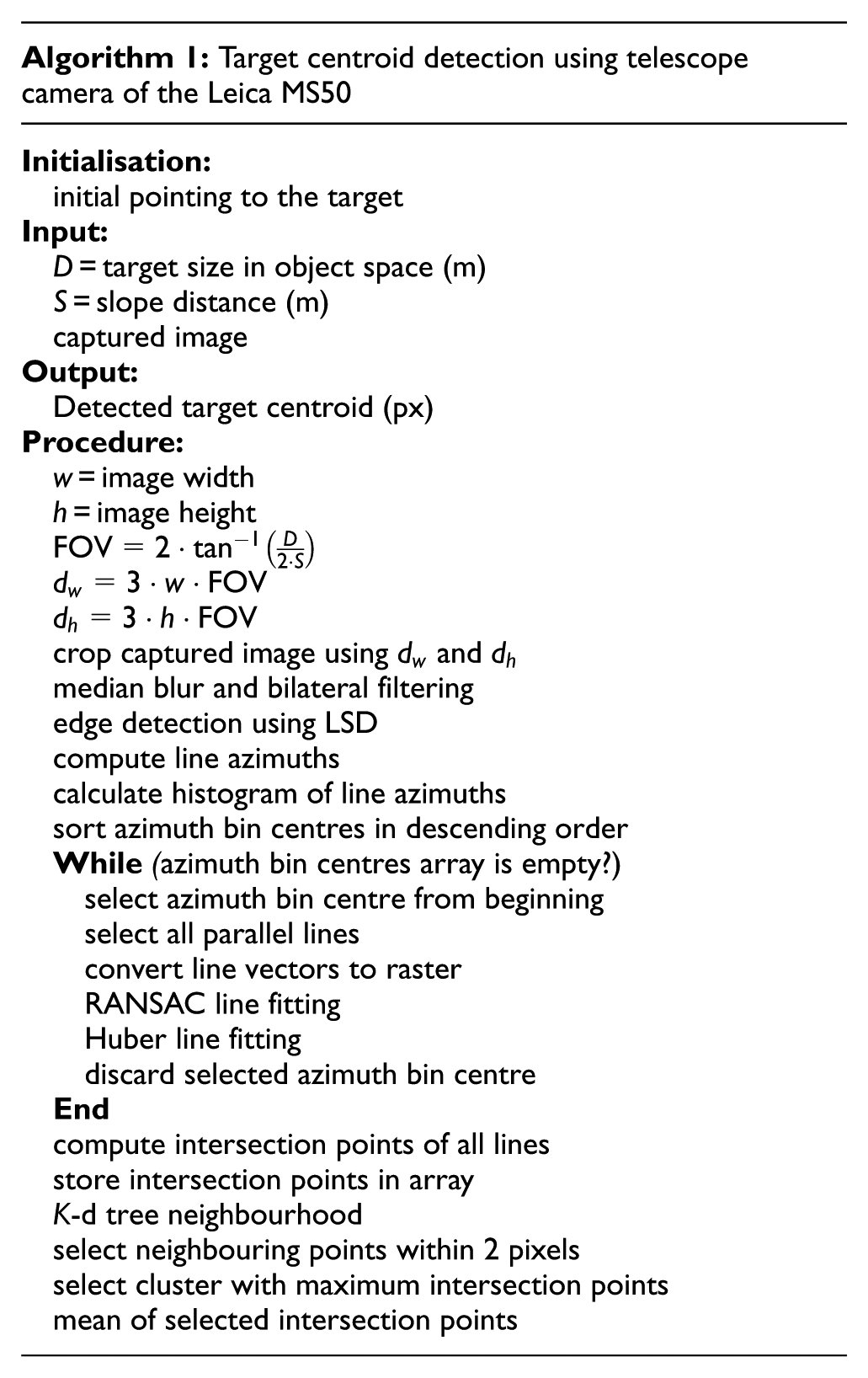
The procedure starts by manual initial pointing of the targets of interest, which is only carried out at the beginning of the measurements. The telescope is then rotated automatically by means of the motorized axes of rotations of the Leica MS50 to the stored positions of the corresponding targets, and images are captured by means of the telescope camera. Subsequently, target centroid detection (see Algorithm 1) is applied, and the telescope is rotated automatically to the detected target centroid to capture images or video frames.
Cropping of the captured images is carried out, taking into account the target object size (in our case 0.06 m), slope distance (here, the maximum slope distance is up to 30 m) and horizontal as well as vertical FOVs of the telescope camera to extract relevant line features of the aforementioned target pattern and to speed up the procedure. Horizontal and vertical FOVs are calculated according to

where
The line segment detector (LSD) algorithm 34 is applied with stable threshold parameters to extract the line features:
The sigma value of the Gaussian filter is set to 0.75;
The bound of quantization error on the gradient norm is set to 2.0;
The gradient angle tolerance is set to 22.5°;
The minimal density of region points in the rectangle is set to 0.7;
The number of bins is set to 1024;
The gradient modulus in the highest bin is set to 255.
Next, the azimuths of the lines are calculated, and the maximum azimuth is selected based on the histogram of the azimuths. Subsequently, those LSD lines within the angle threshold of 15° from the maximum azimuth direction are selected. A random sample consensus (RANSAC) algorithm is applied to the selected lines to fit the optimal line and to get rid of falsely detected parallel lines. To extract lines more accurately, the Huber-robust line fitting algorithm in Kaehler and Bradski 35 with specified buffer width from each side of the fitted RANSAC line is applied. The neighbouring intersection points within 2 px from each intersection point are selected by means of the K-d tree neighbourhood algorithm. Finally, the maximum intersection point cluster is selected and their mean yields the final intersection point (Algorithm 1; see Omidalizarandi et al. 26 for further information).
Calibration of the optical measurement system
The displacement time series for the captured images of the Leica MS50 is produced by subtracting the extracted target centroids at different epochs of time. Subsequently, the calculated displacements in the pixel unit are converted to the more meaningful metric unit by means of the calibration parameters. The calibration consists of an internal calibration of the telescope camera of the Leica MS50 (regarding focal length, principal point and radial and tangential distortions) and an internal calibration of the error sources of the Leica MS50 measurements (including the zero offset for distance measurements or horizontal collimation error, vertical index error, tilting axis error and compensator index error of angular measurements). As mentioned previously, the FOV is reduced by

where
As we can see from Figure 4, the differences in the amplitudes for all three sensors are at a sub-millimetre-level accuracy. However, the time synchronization is still a challenge and needs to be performed precisely. In this work, the time synchronization is performed merely for the controlled excitation in the laboratory environment by changing the frequency and amplitude of the PSVC and by fitting the time series of all three sensors at a point of change. Subsequently, as we can also see in Figure 4, the synchronization was not achieved perfectly. However, time synchronization is not in the focus of this research and will be investigated as part of future research.

Displacement time series for the PSVC, the LT and the Leica MS50 at 3 Hz and distance of 7.52 m.
The vertical angular conversion factor of the telescope camera of the Leica MS50 is calibrated to convert pixel quantities to metric quantities. The calibration is started by designing a coded target pattern in the software AutoCAD 2016 in the two paper sizes

The coded target images captured using the telescope camera of the Leica MS50 at distances of 30.39 m (left) and 14.68 m (right).
The next step is to extract the target centroids of the coded target pattern images captured at different distances up to approximately 30 m and to assign them the unique IDs. To extract a target centroid, median blur and bilateral filtering are first applied to reduce the noise and to preserve the sharp edges of the images. The canny edge detector 36 is then applied to extract the edges. The inner circular part of the coded target is extracted by means of the Hough circle transform (HCT). 35 To find the circles based on the HCT, the circle radius is approximately calculated using equations (1) and (3)–(5) 26


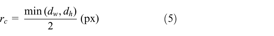
where
Next, the ellipse fitting in a least-squares sense is applied to the concentric edge contours with detected Hough circles. In order to assign a unique ID to each target and to detect coded targets, template matching is applied by their comparisons with the designed coded targets. Finally, the vertical angular conversion factor is calculated based on the equations


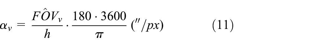
where
The MATLAB functions polyfit and polyval are used, respectively, to fit a best line to the psy calculated for different slope distances and to evaluate it at specified distances. Figure 6 (left) depicts the psy values calculated for different slope distances, and Figure 6 (right) zooms in around the slope distance of 15 m.

Depiction of the pixel sizes of the captured images in the direction of y axis with respect to the slope distances (left) and the magnification of the area highlighted by the circle (right).
The value 1.9583 (″/px) is obtained from the evaluation of the previous equations for calculation of the
Displacement and vibration analysis
The discrete Fourier transform (DFT) is typically applied to estimate the amplitude and frequency of oscillating objects, such as bridge structures. It might achieve reasonable results while the measurements are less contaminated with the coloured noise. To tackle this problem and to estimate the amplitude and frequency even in the case of high coloured measurement noise, we proposed a robust and consistent procedure which can be extended and used for any type of measurement, particularly the vision-based measurement system, to obtain the highly accurate results. In this research, we utilize the captured video frames from the telescope camera of the Leica MS50 for displacement and vibration analysis of a footbridge structure.
We use a simple harmonic motion to perform the displacement measurements, which means that the acceleration measurement is directly proportional to its displacement from the equilibrium position. In addition, the acceleration is directed towards the equilibrium position. 37 Subsequently, the extracted target centroids from video streams of the Leica MS50 or the 3D coordinates from the LT are always averaged over a specified period of time to define the equilibrium position. We can calculate the displacement and acceleration for Leica MS50 measurements using the equations


where
To compare the Leica MS50 and the LT, we can calculate the displacements for the Leica MS50 measurements based on equation (12) and then input the displacements to equation (15) to calculate the amplitude (mm) and the frequency (Hz), respectively. Concerning the comparison of the Leica MS50 and the PSVC, we note that the output of the latter consists of acceleration measurements; we can calculate accelerations for the Leica MS50 measurements based on equation (13) and then use equation (15) to calculate the amplitude (m/s2) and the frequency (Hz). However, it is also possible to calculate displacements from the acceleration measurements via double integration from equation (15).
To estimate the frequency, merely pixel differences are sufficient to derive reasonable results due to the linearity property

of the Fourier transform.16,38 Despite this possibility, we performed both displacement and vibration analysis in metric unit measurements.
We modelled the given vibration measurements

The frequencies

in which the coefficients

where the lag operator
Within iteration step

which depend on currently available initial or estimated parameter values
The M-step can be carried out by solving the four parameter groups individually. First, the parameters
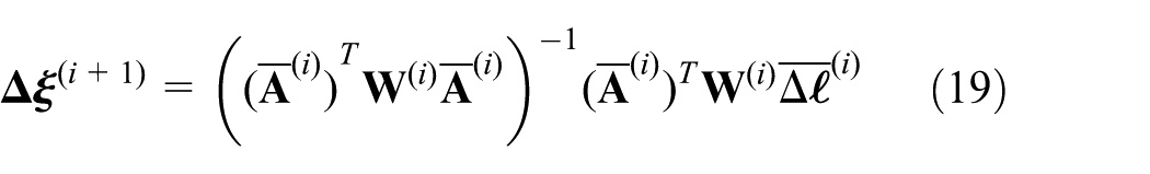
with reduced observations


A Gauss–Newton step with step size

and this solution yields the estimated coloured noise residuals

and then compute the solution of the normal equations with respect to the AR coefficients

Here, we need to check whether all roots of

Finally, to estimate the degree of freedom of the underlying t-distribution, we determine the zero of the equation

where the weights
Experiments and results
We performed accurate displacement and vibration analysis using video streams from the telescope camera of a Leica MS50 with a practical sampling frequency of 10 Hz. Experiments were performed for two case studies under (1) a controlled laboratory environment and (2) an uncontrolled real-world situation observing a footbridge structure using the telescope camera of Leica MS50. Furthermore, an LT and a PSVC were used as two highly accurate reference sensors with a sampling frequency of 200 Hz for the validation purposes. Alternatively, the calculated natural frequencies of the footbridge structure based on the FEM were utilized for a validation.
The primary step to perform a displacement and vibration analysis based on the video frames of the Leica MS50 was to select an optimal passive target pattern and to extract its centroid with high accuracy at different epochs of time. Next, the vertical angular conversion factor of the telescope camera of the Leica MS50 was calibrated, which allows us to convert derived displacements from the pixel unit to the metric unit. In addition, the Fourier series (equation (15)) as a linear regression model and an AR process (equation (16)) as a coloured noise model were employed to estimate amplitudes and frequencies with high accuracy, assuming the white-noise components to follow a scaled t-distribution with an unknown scale factor and unknown degree of freedom. To estimate the model parameters by means of the GEM algorithm described in the preceding section, the number
Example based on the shaker vibration calibrator
The controlled excitations were performed at the laboratory of the Geodetic Institute Hannover (GIH) of the Leibniz Universität Hannover (LUH; see Figure 7, right) by means of the Leica MS50, LT, PSVC and IMU Brick 2.0 (which constitutes a low-cost accelerometer). The analysis of the IMU Brick 2.0 measurements is beyond the scope of this article and will be carried in our future research. As can be seen from Figure 7 (left), the optimal passive target pattern as proposed by Omidalizarandi et al.
26
oscillates as part of the PSVC and is simultaneously measured through video streaming by means of the telescope camera of the Leica MS50. The PSVC contains a PCB ICP quartz reference accelerometer, which outputs highly accurate acceleration data. Specifically, the oscillation frequencies of 2, 3 and 4 Hz with an amplitude of 0.3 m/s2 were adjusted throughout two sensitive dials. Each frequency was measured for a about 7 min by all four sensors. However, since the sampling frequency of the Leica MS50 is only 10 Hz in practice, the frequencies of higher than 5 Hz could not be captured by the Leica MS50 (in view of the Nyquist sampling theorem). To perform measurements with the LT, a Leica red-ring reflector (RRR) 0.5

Vibration analysis of a controlled excitation based on acceleration measurements from the PSVC 9210D, video streams from the telescope camera of the Leica MS50, 3D coordinates from the LT Leica AT960-LR and acceleration measurements from the IMU Brick 2.0.
Figure 8 shows the displacement time series of the extracted target centroid with respect to the mean of the extracted centroids throughout time in both millimetre and pixel units at 2 Hz frequency and a slope distance of 5.3616 m. In addition, the first 20 s of the Leica MS50 data and the first 5 s of the LT and PSVC data were discarded as transient oscillations.

Displacement time series of the extracted target centroid for the telescope camera images of the Leica MS50 at 2 Hz and a distance of 5.3616 m.
Figure 9 depicts the DFT of the video streams from the Leica MS50 at a distance of 5.3616 m, where the frequency induced by the PSVC was 2 Hz. This frequency is clearly associated with the maximum amplitude. Figure 10 shows the target centroid extracted from the Leica MS50 video streams alongside the adjusted Fourier model at 2 Hz for a 5 s time section.

Typical discrete Fourier transform of one segment of the Leica MS50 dataset at distance of 5.3616 m, showing the main amplitude at 2 Hz.

Typical section of the Fourier model (solid line) fitted to the given measurements of the Leica MS50 dataset (stars) at 2 Hz within 5 s.
Figure 11 shows the estimated coloured noise residuals and the decorrelated residuals of the Leica MS50 dataset, resulting from the filtering (equation (17)) of the former residuals by means of the inverted estimated AR model. Figure 12 shows the adequacy of the estimated AR coloured noise models in the light of an accepted (periodogram-based) white noise. 39
Typical segment showing the estimated coloured noise residuals and the decorrelated residuals of the Leica MS50 dataset at 2 Hz and a distance of 5.3616 m.
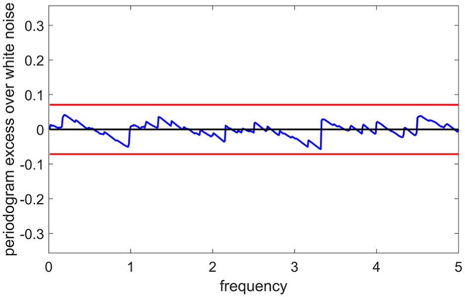
Excess of the estimated periodogram of the decorrelated (i.e. estimated white noise) residuals of the Leica MS50 dataset at 2 Hz and a distance of 5.3616 m for the AR(25) model (jagged line) with respect to the theoretical white noise periodogram (horizontal centred line) and 99% significance bounds (horizontal bounded lines).
The DFT is shown in Figure 13, which reveals two main amplitudes at 1.25 and 2.5 Hz to shed further light on the impact of the image motion error (see Figure 14) on the estimation of the frequency. In addition, Figure 15 shows a higher coloured noise level in comparison to Figure 11, which proves the existence of the image motion errors throughout this time interval of the experiment.
Typical discrete Fourier transform of one segment of the Leica MS50 dataset at a distance of 22.6635 m, showing two main amplitudes at 1.25 and 2.5 Hz.

Displacements of the extracted target centroid for telescope camera images of Leica MS50 at 2 Hz and a distance of 22.6635 m.

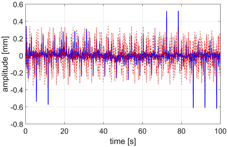
Typical segment showing the estimated coloured noise residuals (dashed line) and the estimated white noise residuals (solid line) of the Leica MS50 dataset at 2 Hz and a distance of 22.6635 m.
Table 1 summarizes the statistics of the displacement and vibration analysis for all three sensors. In most cases, the frequencies and amplitudes estimated from the Leica MS50 measurements are very close to those resulting from the two highly accurate reference sensors (LT and PSVC). The estimated degrees of freedom of the t-distribution underlie the white noise components. Concerning the LT and the PSVC measurements, these estimates are roughly between 14 and 60, indicating a rather close approximation of a normal distribution. By contrast, the estimated degrees of freedom regarding the Leica MS50 measurements are in the range of 2–4.5, for which values the t-distribution has substantial tails; we thus found a large number of outliers in the measurement noise of that sensor.
Statistics of the displacement and vibration analysis for the Leica MS50, LT and PSVC measurements with an AR order of

LT: laser tracker; PSVC: portable shaker vibration calibrator; AR: autoregressive.
Furthermore, the results show that the highest white noise test acceptance rate (100%) was obtained for the PSVC measurements, for which an AR order of
Table 2 summarizes the statistics of the displacement and vibration analysis for all three sensors without AR processing to give an impression about strength of the developed algorithm. In addition, the degree of freedom was fixed to 120, which stands for the t-distribution, approximating the normal distribution as described in Abramowitz and Stegun 40 and Koch. 41 As we expected, the absolute deviations from the PSVC without the AR processing are not significant and has less coloured measurement noise, as the estimated degree of freedoms indicate approximately the normal distribution (see Table 1). In addition, the absolute deviations for the LT measurement without the AR processing are slightly larger than those including AR processing. However, the absolute deviations for the Leica MS50 without the AR processing are mostly and significantly larger than those included in the AR processing. In addition, as the estimated degrees of freedom for the Leica MS50 data are represented by a range of 2–4.5 (see Table 1), it proves the existence of numerous outliers in the dataset. Subsequently, by ignoring the AR processing within the robust estimation procedure developed for the Leica MS50, the results in some cases do not prove to be reliable or accurate enough.
Statistics of the displacement and vibration analysis for the Leica MS50, LT and PSVC measurements without AR model and

LT: laser tracker; PSVC: portable shaker vibration calibrator; AR: autoregressive.
Example based on real application of a footbridge structure
An uncontrolled excitation of a footbridge structure with a length of 27.051 m and a width of 2.72 m close to the GIH (see Figure 16) was measured using the Leica MS50 and LT. The measurements were carried out for the first quarter and the middle of the footbridge structure (marked by the circles in Figure 16). Alternatively, the known natural frequencies of the footbridge structure were utilized for a validation. They were calculated based on the FEM analysis of a design model of the footbridge structure, which was carried out by the Institute of Concrete Construction of the LUH. According to that, the vertical natural frequencies of the footbridge structure are 3.642 and 13.294 Hz, the longitudinal and the lateral natural frequencies are 2.295 and 7.053 Hz, and the torsional natural frequencies are 3.759 and 11.828 Hz, respectively. As we can see in Figure 16, the Leica MS50 and the LT are located at the footpath close to the side of the footbridge structure. Regarding the natural frequencies, we could only detect the vertical natural frequency of 3.642 Hz and could not detect another one with the value of 13.294 Hz due to the low practical sampling frequency of 10 Hz of the Leica MS50 and in view of Nyquist sampling theorem. On the other hand, it might be necessary to set-up the Leica MS50 in a place, where it can measure the passive targets perpendicularly to detect the longitudinal and lateral natural frequencies of the footbridge structure. However, this was not the case in our measurement campaign and we could not detect those natural frequencies either.
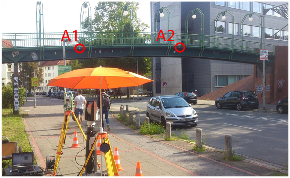
Vibration analysis of the footbridge structure using the telescope camera of the Leica MS50 to measure the passive targets attached to the side of the footbridge (areas highlighted by the circles) and using the LT to measure an attached corner cube reflector close to the aforementioned passive targets.
Figures 17 and 18 show the DFT results for the Leica MS50 measurement at Points A1 and A2, respectively. In addition, Figure 19 shows the DFT result at point A1 for the LT measurement as well. Since the time synchronization needed to be performed between the Leica MS50 and the LT measurements and was not the case in our measurement campaign, the one-to-one comparison between the results of the aforementioned sensors does not make sense. However, we can rely on the FEM results of the design model of the footbridge structure for the validation in this case study. As can be seen from Figures 17 and 19, the DFT results at point A1 show the frequency of 4.07 Hz with the maximum amplitude of 0.07 mm, which was captured by the Leica MS50 measurements, whereas the frequency of 4.06 Hz with the maximum amplitude of 0.0497 mm was obtained for the LT measurements. However, the results from the proposed approach show the frequencies of 4.0768 and 4.0631 Hz with the maximum amplitudes of 0.0433 and 0.0462 mm for the Leica MS50 and LT measurements, respectively. However, the DFT result in Figure 18 at point A2 shows the frequencies of 3.65 and 4.1 Hz with the maximum amplitudes of 0.079 and 0.055 mm, respectively. However, the proposed approach shows the frequencies of 3.6451 and 4.0978 Hz with the maximum amplitudes of 0.051 and 0.0367 mm, respectively, which are comparable to those calculated from the FEM with the frequency of 3.642 Hz, and these findings demonstrate the correctness of our calculations. The higher frequency of approximately 4.07 Hz obtained might be due to either modulating the higher frequency of 13.294 Hz or an additional vibration produced by people passing across the footbridge structure and the latter not reaching a stable situation at the time of measurement.

Point A1: Typical discrete Fourier transform of one segment of the Leica MS50 dataset at a distance of 16.5 m from footbridge structure, showing the main amplitude of 0.07 mm at a frequency of 4.07 Hz.
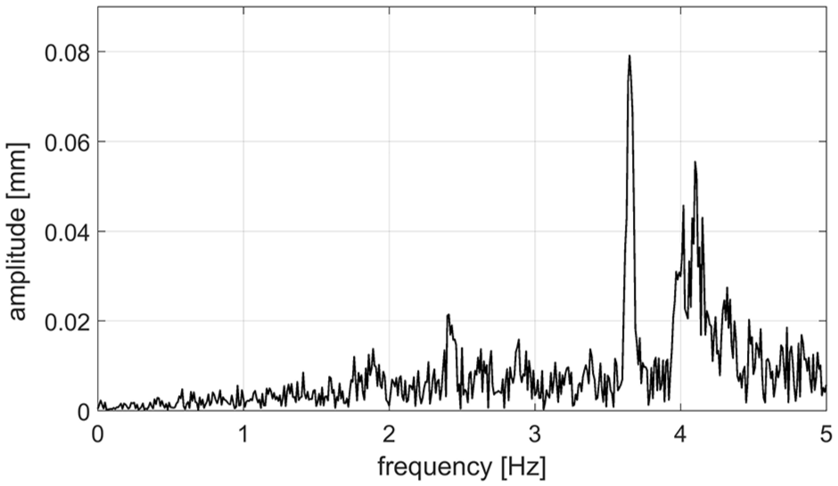
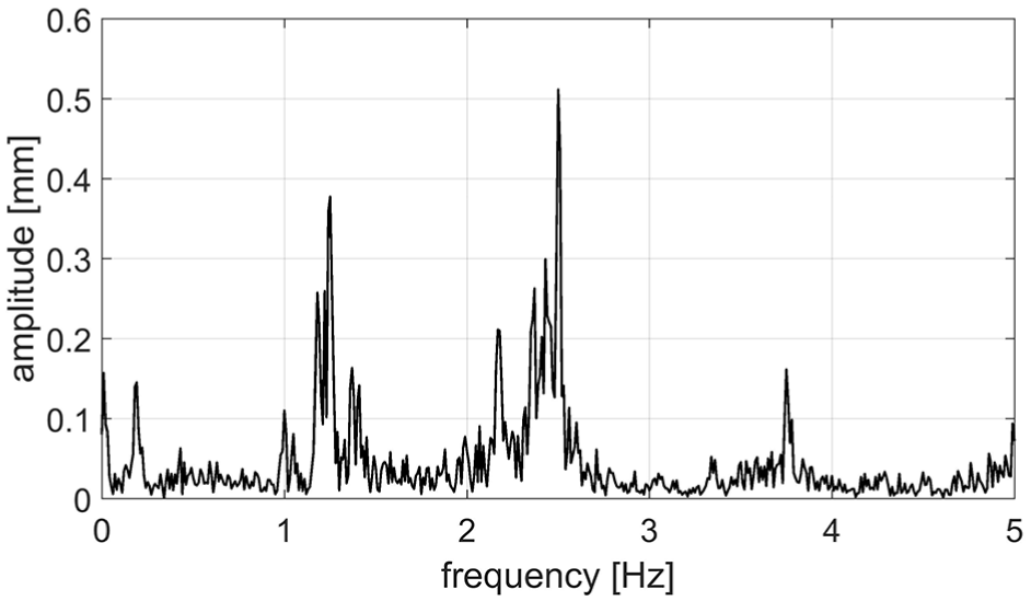
Point A2: Typical discrete Fourier transform of one segment of the Leica MS50 dataset at a distance of 20.01 m from footbridge structure, showing the main amplitudes of 0.079 and 0.055 mm at frequencies of 3.65 and 4.1 Hz, respectively.

Point A1: Typical discrete Fourier transform of one segment of the LT dataset at a distance of 16.499 m from the footbridge structure, showing the main amplitude of 0.0497 mm at a frequency of 4.06 Hz.
In addition, Figures 20–22 illustrate the estimated coloured noise residuals and the decorrelated (i.e. estimated white noise) residuals for the Leica MS50 at the two points of A1 and A2 in addition to the LT measurements, respectively. We should mention that the LT measurements of the bridge structure were performed with a corner cube reflector of lesser quality than for measurements within the laboratory experiment. Consequently, a high level of noise in the displacements for some segments appears in the results, which we can be improved in our future work by employing a corner cube reflector of a better quality. In addition, we could even improve the Leica MS50 results by taking angular tilt axis errors into account and by avoiding the very minor shaking of the instrument.

Point A1: Typical segment showing the estimated coloured noise residuals (dashed line) and the estimated white noise residuals (solid line) of the Leica MS50 dataset with the main amplitude at 4.07 Hz for the footbridge structure.

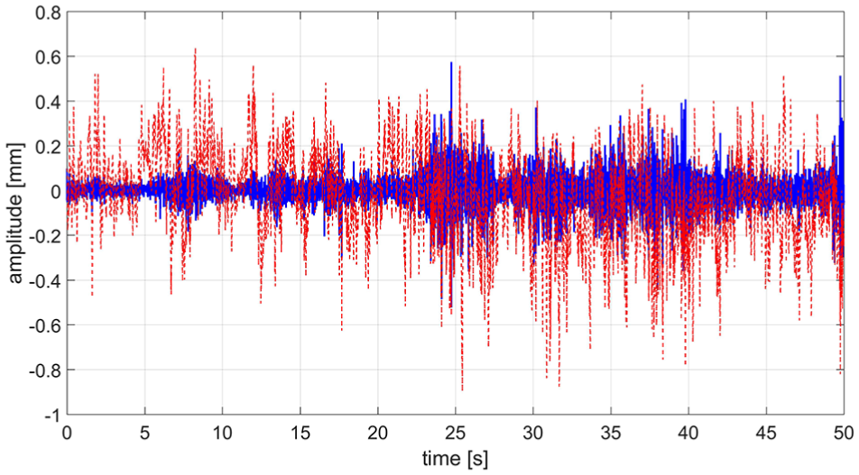
Point A2: Typical segment showing the estimated coloured noise residuals (dashed line) and the estimated white noise residuals (solid line) of the Leica MS50 dataset with the main amplitudes at frequencies of 3.65 and 4.1 Hz for the footbridge structure.
Point A1: Typical segment showing the estimated coloured noise residuals (dashed line) and the estimated white noise residuals (solid line) of the LT dataset with the main amplitude at 4.06 Hz for the footbridge structure.
Conclusion
A robust and consistent procedure was proposed to perform an accurate displacement and vibration analysis of a footbridge structure using an IATS (here, Leica MS50). The Leica MS50 benefits accurate distance measurements to the object in addition to the captured video streams with a practical sampling frequency of 10 Hz using an embedded on-axis telescope camera. The experiments were carried out for two case studies under a controlled excitation in the laboratory environment and an uncontrolled excitation of a footbridge structure. In a first case study, the results were validated by means of two highly accurate reference measurement systems, namely, the portable shaker vibration calibrator 9210D (with a sampling frequency of 200 Hz) and the Leica AT960-LR LT (with a sampling frequency of 200 Hz). In the second case study, the validation was performed based on the known natural frequencies of the footbridge structure calculated from the FEM analysis. In addition, the LT measurement was also used for a validation.
To extract target centroid from video streams of the Leica MS50, the feasibility of an optimal passive target pattern including four intersected lines and its accurate and reliable detection approach, proposed in Omidalizarandi et al., 26 were investigated at different epochs of time as a preliminary step. Subsequently, the vertical angular conversion factor was calibrated in the laboratory environment to convert derived displacements from the pixel unit to the metric unit.
To estimate amplitudes and frequencies for all three sensors with high accuracy, vibration measurements either in the length unit or the acceleration unit were input to the Fourier series as a linear regression model comprising a sum of sinusoids and additive random deviations. Furthermore, the coloured measurement noise was decorrelated through a covariance-stationary AR process of an order 25, assuming the white noise components to independently follow a central and scaled t-distribution with an unknown scale factor and unknown degree of freedom. At the end, model parameters were estimated by means of the GEM algorithm as described in Alkhatib et al. 30 The unknown frequencies were initiated by means of notable maximum amplitudes within the DFT of the data to perform adjustment of the combined observation model for a footbridge application.
The results indicate that the estimated frequencies and amplitudes from the Leica MS50 measurements were very close to those resulting from the two highly accurate reference sensors (LT and PSVC) in the laboratory environment and to those resulting from the FEM analysis and the LT for the real application of the footbridge structure. It was shown that the DFT results and our proposed approach achieved approximately similar results when estimating the frequencies. However, the results for the amplitudes varied from minor to significant changes depending on the coloured noise behaviour of the measurements. To show the strength of the proposed approach, the estimated results were compared in two cases of the AR model in the order of 25: with an unknown degree of freedom and without the AR process considering a constant degree of freedom of 120, which is close approximation of a normal distribution.
The estimated degrees of freedom of the t-distribution, in the case of considering the AR model order of 25, reveals that the LT and the PSVC measurements are a rather close approximation of a normal distribution, while, by contrast, the estimated degrees of freedom regarding the Leica MS50 measurements with substantial tails show a large number of outliers in the measurement noise of that sensor. Moreover, the results show that the highest white noise test acceptance rate (100%) was obtained for the PSVC measurements. The LT measurements also produced relatively high acceptance rates in comparison to the PSVC data. However, the acceptance rates regarding the Leica MS50 measurements fluctuate between 25% and 75%, so that the adjusted coloured noise model is clearly inadequate for a number of analysed segments. Furthermore, the image motion error for some video frames derived from a weak PC performance or delay in the data transmission procedure from the Leica MS50 to the PC has a significant influence on the estimated frequencies and amplitudes and shows a higher coloured noise level compared to the good quality video frames captured. In summary, the results show the feasibility of Leica MS50 for an accurate displacement and vibration analysis of the footbridge structure for frequencies less than 5 Hz (in view of the Nyquist sampling theorem).
In our future work, we will measure the minor shaking of the Leica MS50 throughout the measurements by continuously reading the tilting axis error of the Leica MS50 using the GeoCOM interface. It might be beneficial to increase the measurement time to obtain more redundant data and to be able to increase AR model order to improve the coloured noise models and the resulting performance of the white noise test. In addition, the proposed approach can be extended to the time-dependant AR model to characterize the coloured noise behaviour of the measurements over time. Furthermore, the time synchronization for the measurements of the sensors can be performed to have a more realistic comparison of the results at a certain point of time. Moreover, we will improve the LT measurements for a footbridge structure by employing a corner cube reflector of a better quality. The internal calibration of the error sources of the Leica MS50 measurements might improve the results. The possibility of performing experiment with the Leica MS60 with a maximum sampling frequency of 20 Hz could also improve the results. Finally, global optimization can be applied for more accurate and reliable results to estimate model parameters with unknown frequencies.
Footnotes
Acknowledgements
The authors would like to acknowledge the Institute of Concrete Construction (Leibniz Universität Hannover) for providing the portable shaker vibration calibrator instrument used within this experiment and for the calculation of the natural frequencies of the footbridge structure based on the FEM. In addition, the authors would also like to acknowledge Falko Klasen, B. Eng., for his assistance with the experiments as part of his master thesis.
Handling Editor: Xiangyang Xu
Declaration of conflicting interests
The author(s) declared no potential conflicts of interest with respect to the research, authorship and/or publication of this article.
Funding
The author(s) disclosed receipt of the following financial support for the research, authorship, and/or publication of this article: The publication of this article was funded by the Open Access fund of Leibniz Universität Hannover. The research presented was partly carried out within the scope of the collaborative project ‘Spatio-temporal monitoring of bridge structures using low cost sensors’ with ALLSAT GmbH, which was supported by the German Federal Ministry for Economic Affairs and Energy (BMWi) and the Central Innovation Programme for SMEs (Grant ZIM Kooperationsprojekt, ZF4081803DB6).