A new Kriging-based DoE strategy and its application to structural reliability analysis

Abstract

As the numerical model of engineering structure becomes more and more complicated and time consuming, efficient structural reliability analysis is badly in need. To reduce the number of calls to the performance function and iterative times during structural reliability analysis, an innovative strategy of the design of experiments (DoE) called Isomap-Clustering strategy is proposed. According to the statistical information provided by Kriging, points with the worst uncertainty for reliability analysis are on the estimated limit state. Therefore, by combining Isomap and k-means clustering algorithm, Isomap-Clustering strategy refreshes the DoE of the Kriging model with a few representative points in the vicinity of the estimated limit state each iteration and iteratively “pushes” the estimated limit state to the real one until a stopping condition is satisfied. By employing the proposed DoE strategy and sparse polynomial-Kriging model, a structural reliability analysis method is constructed, whose stopping criterion is defined by derivation. Three examples are studied. Results show that the proposed method can lower the number of calls to the performance function and remarkably reduces the iterations of structural reliability analysis.

Introduction

The input variables of structures in engineering are often influenced by kinds of randomness. It is necessary to analyze structural reliability by treating inputs as random variables. For a given structure, its performance function G( x ) divides the input space into two domains: the safe domain G( x ) > 0 and the failure domain G( x ) ≤ 0. The boundary of them (G( x ) = 0) is the limit state. The failure probability of the studied structure can be defined as

$$P_f=\underset{G(\mathit{x})\le 0}{\int }f(\mathit{x})\mathrm{d}\mathit{x}$$

(1)

where x is a realization of M-dimension random input vector ( X  = [x₁, x₂, …, x_M]^T) and f( x ) is the joint probability density function (PDF) of X . The main task of structural reliability analysis is to perform the integral of equation (1), which is troublesome for engineering problems with time-consuming G( x ). Several kinds of methods, including the first-order reliability method (FORM) and second-order reliability method (SORM), ¹ random simulation–based methods,^2,3 and surrogate model–based methods,^4,5 have already been developed.

The performance function is usually implicit in engineering, which restricts the application of FORM and SORM. As the most robust method, Monte Carlo simulation (MCS) could meet any accuracy requirement theoretically. ⁶ However, it needs to call the performance function too many times, which is usually impractical to implement. Some alternative simulation techniques, including importance sampling (IS),^7,8 line sampling (LS),^9,10 and subset simulation (SS), ¹¹ are constructed. When structural numerical model needs hours, even days, to calculate once, the existing variance reduction methods are still not efficient enough. In recent years, surrogate models, mainly including polynomial response surface,^12,13 support vector machine (SVM), ¹⁴ neural network, ¹⁵ and Kriging, ¹⁶ are widely used. Surrogate model–based methods construct an explicit expression ( $\hat{G}(\mathit{x})$ ) as the approximation of G( x ) and then estimates the target failure probability by replacing G( x ) with $\hat{G}(\mathit{x})$ in equation (1). This article focuses on Kriging-based reliability analysis method. Compared with other surrogate models, Kriging is an interpolation model and provides an accuracy measure of the predictor, which is its most important advantage. It is widely employed in structural reliability analysis,^5,17–19 global optimization,^20,21 and sensitivity analysis.^22,23

For reliability analysis applications, it is enough to accurately approximate the performance function in the vicinity of the limit state rather than in the whole space of inputs. Therefore, several adaptive DoE strategies are constructed, which aim to efficiently improve the Kriging-based estimate of the limit state and perform the structural reliability analysis by calling to the performance function as fewer times as possible. Inspired by the expected improvement function (EIF) proposed by Jones et al. ²⁰ for global optimization, Bichon et al. ²⁴ propose the expected feasibility function (EFF) to measure how close an untried point is to the limit state and define the next best point of the Kriging model as the maximum point of EFF. Echard et al. ¹⁷ develop a reliability analysis method by combining the Kriging model with MCS (AK-MCS), in which the best next point is defined according to their proposed learning function U. The learning function U measures the probability that the Kriging model wrongly predicts the sign of the performance value at a point. It is also employed by AK-IS, ²⁵ AK-SS, ²⁶ and AK-SSIS. ¹⁹ Lv et al. ¹⁸ and Yang and colleagues^27–29 measure the epistemic uncertainty of the sign of the performance value from different perspective and develop their learning functions H and expected risk function (ERF), respectively. Recently, Sun et al. ³⁰ propose an innovative learning function least improvement function (LIF) which quantitatively measures how much an untried point could improve the Kriging-based estimate of the failure probability.

These learning function–based adaptive DoE strategies mentioned above are able to efficiently enhance the accuracy of the Kriging model. However, because the Kriging model is refreshed with only one point every iteration, they always need many iterative steps to meet a stopping criterion. As the development of hardware, parallel computing is usually available in engineering, which is helpful to remarkably reduce the number of iterations.

To make the best of hardware resources and further improve the computational efficiency of structural reliability analysis with time-consuming performance function, an innovative adaptive DoE strategy of the Kriging model, named as Isomap-Clustering strategy, is proposed, which combines Isomap (a nonlinear dimensionality reduction method) with k-means clustering. The proposed strategy is designed to refresh the Kriging model with a few points each iteration. As the signs of performance values of points on the estimate of the limit state estimate ( $\hat{G}(\mathit{x})=0$ ) are with the most uncertainty, the proposed strategy selects “representative points” in the vicinity of $\hat{G}(\mathit{x})=0$ to enhance the accuracy of the Kriging model. To realize the goal, Isomap maps the candidate points randomly generated to lower space, and then, k-means clustering algorithm is employed to find the cluster centers of the mapped points. Representative points can be obtained by one-to-one mapping of Isomap dimensionality reduction. In this way, it is avoided that any two of the representative points are too close to each other. A Kriging-based reliability analysis procedure is developed mainly based on the proposed Isomap-Clustering strategy. And the basic function of the Kriging model is sparse polynomial, which is constructed according to least angle regression (LAR) and Akaike information criterion (AIC).

The remainder of this research is organized as follows. Section “Sparse polynomial-Kriging” introduces the basic theory of Kriging and the selection procedure of its basic function. Section “The Isomap-Clustering strategy” details the proposed Isomap-Clustering strategy, which is followed by the Kriging-based reliability analysis method. Section “Numerical applications” studies two analytical examples and one truss structure to demonstrate the advantage of the proposed adaptive DoE strategy. Section “Conclusion” presents the conclusion.

Sparse polynomial-Kriging

The Kriging model

Kriging developed by Krige for geostatistics and improved by Matheron ³¹ is a nonlinearity interpolation meta-model. It supposes that the deterministic function needed to be approximated consists of two parts, that is, a regression model and a random function

$$G(\mathit{x})=\sum _{h=1}^p{\beta }_h{g}_h(\mathit{x})+z(\mathit{x})={\mathit{g}}^{\mathrm{T}}(\mathit{x})\mathit{\beta }+z(\mathit{x})$$

(2)

where g_h( x ) (h = 1,2, …, p) is the regression basis, which is discussed in section “Basic function of the Kriging model.”z( x ) is a Gaussian stochastic process with zero mean, whose covariance is defined as

$$\mathrm{Cov}[z({\mathit{x}}_i),z({\mathit{x}}_j)]={\sigma }^{2}R({\mathit{x}}_i,{\mathit{x}}_j;\mathit{\theta })$$

(3)

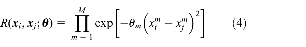
where σ² is the variance of z( x ). R( x _i , x _j ; θ ), the correlation coefficient between z(x_i) and z(x_j) with parameter θ , is the Gaussian correlation function generally

$$R({\mathit{x}}_i,{\mathit{x}}_j;\mathit{\theta })=\underset{m=1}{\overset{M}{\Pi }}\exp [-{\theta }_m{(x_i^m-x_j^m)}^2]$$

(4)

where $x_i^m$ is the mth component of x _i .

Given a DoE S _DoE = [x₁, x₂, …, x_N], and the corresponding performance values Y = [y₁, y₂, …, y_N]^T, the unknown parameters β , σ², and θ in equations (2)–(4) can be estimated by maximum likelihood estimation

$$maxL(\mathit{\theta })=-(N\ln ({\hat{\sigma }}^2)+\ln [det(\mathit{R})])$$

(5)

where

$$\begin{array}{c}{\hat{\sigma }}^2=\frac{1}{N}(\mathit{Y}-{\mathit{G}}^{\mathrm{T}}\mathit{\beta }{)}^{\mathrm{T}}{\mathit{R}}^{-1}(\mathit{Y}-{\mathit{G}}^{\mathrm{T}}\mathit{\beta })\hfill \\ \mathit{\beta }=({\mathit{G}}^{\mathrm{T}}{\mathit{R}}^{-1}\mathit{G}{)}^{-1}{\mathit{G}}^{\mathrm{T}}{\mathit{R}}^{-1}\mathit{Y}\hfill \\ \mathit{G}=[\mathit{g}({\mathit{x}}_1),\mathit{g}({\mathit{x}}_2),\dots ,\mathit{g}({\mathit{x}}_N){]}^{\mathrm{T}}\hfill \\ \mathit{R}={(R({\mathit{x}}_i,{\mathit{x}}_j;\mathit{\theta }))}_{N\times N}\hfill \end{array}$$

(6)

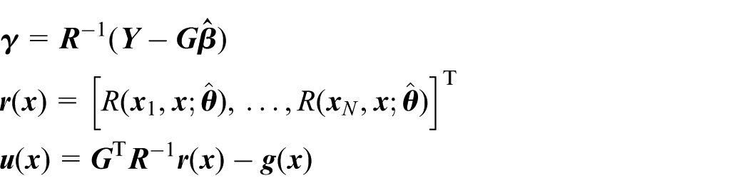
The optimum estimations of β , σ², and θ obtained from equation (5) are denoted by $\hat{\mathit{\beta }},{\hat{\sigma }}^2,\hat{\mathit{\theta }}$ , respectively. The best linear predictor at x reads

$$\hat{G}(\mathit{x})={\mathit{c}}^{\mathrm{T}}(\mathit{x})\mathit{Y}$$

(7)

The error of equation (7) is

$$\begin{array}{cc}\multicolumn{1}{c}{\hat{G}(\mathit{x})-G(\mathit{x})}& ={\mathit{c}}^{\mathrm{T}}(\mathit{x})\mathit{Y}-G(\mathit{x})\hfill \\ \multicolumn{1}{c}{}& ={\mathit{c}}^{\mathrm{T}}(\mathit{x})\mathit{Z}-z+({\mathit{G}}^{\mathrm{T}}\mathit{c}(\mathit{x})-\mathit{g}(\mathit{x}){)}^{\mathrm{T}}\hat{\mathit{\beta }}\hfill \end{array}$$

where

$$\mathit{Z}=[z_1,z_2,\dots ,z_N{]}^{\mathrm{T}}$$

The minimum variance unbiased estimator of G( x ) is

$${\mu }_G(\mathit{x})=\widehat{G}(\mathit{x})={\mathit{g}}^{\mathrm{T}}(\mathit{x})\widehat{\mathit{\beta }}+\mathit{r}{(\mathit{x})}^{\mathrm{T}}\mathit{\gamma }$$

(8)

$${\sigma }_G^2(\mathit{x})={\hat{\sigma }}^2(1+{\mathit{u}}^{\mathrm{T}}(\mathit{x}){({\mathit{G}}^{\mathrm{T}}{\mathit{R}}^{-1}\mathit{F})}^{-1}\mathit{u}(\mathit{x})-{\mathit{r}}^{\mathrm{T}}(\mathit{x}){\mathit{R}}^{-1}\mathit{r}(\mathit{x}))$$

(9)

where

$$\begin{array}{c}\mathit{\gamma }={\mathit{R}}^{-1}(\mathit{Y}-\mathit{G}\hat{\mathit{\beta }})\hfill \\ \mathit{r}(\mathit{x})={[R({\mathit{x}}_1,\mathit{x};\hat{\mathit{\theta }}),\dots ,R({\mathit{x}}_N,\mathit{x};\hat{\mathit{\theta }})]}^{\mathrm{T}}\hfill \\ \mathit{u}(\mathit{x})={\mathit{G}}^{\mathrm{T}}{\mathit{R}}^{-1}\mathit{r}(\mathit{x})-\mathit{g}(\mathit{x})\hfill \end{array}$$

So, the real performance value at x subjects to normal distribution, whose mean and standard deviation are ${\mu }_G(\mathit{x})$ and ${\sigma }_G^2(\mathit{x})$ , respectively

$$G(\mathit{x})~N({\mu }_G(\mathit{x}),{\sigma }_G^2(\mathit{x}))$$

(10)

Bichon et al. ²⁴ show the detailed theory of the Kriging model.

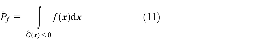
The failure probability of studied structure can be estimated as

$${\hat{P}}_f=\underset{\hat{G}(\mathit{x})\le 0}{\int }f(\mathit{x})\mathrm{d}\mathit{x}$$

(11)

MCS is adopted here to perform the multiple integration of equation (11)

$${\hat{P}}_f\approx \frac{1}{N_{\mathrm{MC}}}\sum _{i=1}^{N_{\mathrm{MC}}}{I}_{\hat{G}<0}\left({\mathit{x}}_{\mathrm{MC},i}\right)$$

(12)

where x _MC , _i (i = 1, 2, …, N_MC) is a sequence of independent identically distributed (i.i.d.) points generated from f( x ) and N_MC is the number of random points. The coefficient of variation of ${\hat{P}}_{\mathrm{f}}$ is

$${\delta }_{\mathrm{MC}}=\frac{\sqrt{\mathrm{var}({\hat{P}}_f)}}{{\hat{P}}_f}=\sqrt{\frac{1-{\hat{P}}_f}{N_{\mathrm{MC}}{\hat{P}}_f}}\approx \frac{1}{\sqrt{N_{\mathrm{MC}}{\hat{P}}_f}}$$

(13)

Basic function of the Kriging model

It is supported that the input random variable X subjects to multivariate standard normal distribution and the components are independent. Otherwise, X is available to exactly or approximately transform into multivariate standard normal distribution.

Regression basis function, g_h( x ) (h = 1, 2, …, p), is generally set to be constant or multivariate polynomial. Gaspar et al. ⁵ assess the accuracy of Kriging model with different basis functions. The effect of the order of basis function shown to be negligible if there are enough DoE points. Higher order of g_h( x ) appears rewarding to the Kriging model in case that the number of points in S _DoE is low, which usually occurs during structural reliability analysis if the performance function is time consuming. However, the number of terms of basic function increases dramatically with the size of X and the order of polynomial, which makes the high order (e.g. cubic) almost unavailable for the Kriging model during reliability analysis. To address such problem, this article constructs the basic function with sparse polynomial, during which LAR ³² and AIC are adopted.

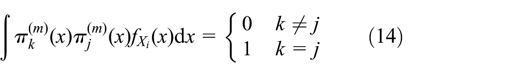
Let ${\pi }_j^{(m)}$ (j = 1,2, …) denotes the complete orthonormal basis of the Hilbert space $L^2(R,f_{X_i})$ , which means that ${\pi }_j^{(m)}$ (j = 1,2,…) is an orthonormal function series in the sense of $f_{X_i}$

$$\int {\pi }_k^{(m)}(x){\pi }_j^{(m)}(x)f_{X_i}(x)\mathrm{d}x=\{\begin{array}{c}0k\ne j\hfill \\ \multicolumn{1}{c}{1k=j}\end{array}$$

(14)

where $f_{X_i}$ is the PDF of X_i (mth component of X ).

A possible complete orthonormal basis of the Hilbert space L²(R, f) (f is the joint PDF of X ) is

$${\psi }_{\mathit{\alpha }}(\mathit{X})=\underset{m=1}{\overset{M}{\Pi }}{\pi }_{{\alpha }_m}^{(m)}(X_m)$$

where α = [α₁, α₂, …, α_M] is a M-dimension vector of natural number. Here, the terms whose total degree | α | = α₁ + α₂ + … + α_M does not exceed a given threshold value T₀ are retained as candidates of the basic function of the Kriging model. The set of candidates of the basic function is denoted by ${\mathrm{A}}^{M,T_0}$

$${\mathrm{A}}^{M,T_0}=\{\mathit{\alpha }\in {\mathrm{N}}^M,|\mathit{\alpha }|\le T_0\}$$

The number of the elements in ${\mathrm{A}}^{M,T_0}$ is P

$$P=\mathrm{card}\left({\mathrm{A}}^{M,T_0}\right)=\left(\begin{array}{c}M+T_0\hfill \\ \multicolumn{1}{c}{T_0}\end{array}\right)$$

(15)

Then, the “complete” design matrix that considers all candidates of the basic function is

$$\begin{array}{c}{\mathit{G}}^{M,T_0}=[{\mathit{\psi }}_{{\mathit{\alpha }}_0},{\mathit{\psi }}_{{\mathit{\alpha }}_2},\dots ,{\mathit{\psi }}_{{\mathit{\alpha }}_{P-1}}]\hfill \\ {\mathit{\psi }}_{{\mathit{\alpha }}_i}=[{\psi }_{{\mathit{\alpha }}_i}({\mathit{x}}_1),{\psi }_{{\mathit{\alpha }}_i}({\mathit{x}}_2),\dots ,{\psi }_{{\mathit{\alpha }}_i}({\mathit{x}}_N){]}^{\mathrm{T}}\hfill \end{array}$$

where ${\mathit{\alpha }}_i\in \mathrm{A}(i=0,1,\dots ,P-1)$ and x _n  ∈  S _DoE (n = 1, 2, …, N).

According to equation (15), the least number of calls to the performance function increases extremely with T₀ if employing all terms in ${\mathrm{A}}^{M,T_0}$ as the basic function of the Kriging model. To overcome the problem, only a part of terms in ${\mathrm{A}}^{M,T_0}$ are retained to build up the sparse polynomial basic function. LAR is employed to provide a number of possible polynomial basis sets that can explain the performance function, and AIC is used to decide which is the optimal. The main steps of the selection of the Kriging basic function are listed as follows:

• Step 1. Set values of parameters concerned, that is, the maximal order of retained polynomial T₀ and the maximal number of terms of the basic function p_max. In this article, T₀ = 3 and p_max = 0.5 card ( S _DoE)

$$H=min\{P,p_{max}\}$$

• Step 2. Initialize all the coefficients of the candidate terms to $a_{{\mathit{\alpha }}_i}=0$ (i = 0, 1, …, P − 1). According to LAR theory, the initial residual equals to the structural response Y .

• Step 3. Find the vector ${\mathit{\psi }}_{\mathit{\alpha }{\prime }_1}$ that maximizes the correlation coefficient between ${\mathit{\psi }}_{{\mathit{\alpha }}_i}$ (i = 0, 1, …, P – 1) and the current residual

$${\mathit{G}}_1={\mathit{\psi }}_{\mathit{\alpha }{\prime }_1}$$

• Step 4. h = 2. Adjust $a_{\mathit{\alpha }{\prime }_1}$ in the direction defined by the least square coefficient of the current residual on G ₁, until another vector ${\mathit{\psi }}_{\mathit{\alpha }{\prime }_2}$ has the same correlation coefficient with the current residual as does G ₁

$${\mathit{G}}_h=[{\mathit{G}}_1,{\mathit{\psi }}_{{\mathit{\alpha }\prime }_2}]\mathrm{and}\mathit{a}=[a_{{\mathit{\alpha }\prime }_1},a_{{\mathit{\alpha }\prime }_2}]$$

• Step 5. h = h + 1. Move jointly a toward its joint least square coefficient of the current residual on G _h – 1 until a vector ${\mathit{\psi }}_{{\mathit{\alpha }}_h}$ has the same correlation coefficient with the current residual as does G _k – 1

$${\mathit{G}}_h=[{\mathit{G}}_{h-1},{\mathit{\psi }}_{{\mathit{\alpha }\prime }_h}]\mathrm{and}\mathit{a}=[a_{{\mathit{\alpha }\prime }_1},a_{{\mathit{\alpha }\prime }_2},\dots ,a_{{\mathit{\alpha }\prime }_h}]$$

• Step 6. Repeat step 5 until h = H.

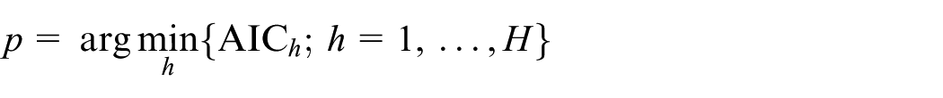
• Step 7. Compute AIC values of G _h (h = 1, …, H)

$$\mathrm{AI}{\mathrm{C}}_h=\mathrm{Nl}\mathrm{n}\left(\mathrm{SS}{\mathrm{E}}_h\right)+2h$$

where

$$\mathrm{SS}{\mathrm{E}}_h={[G_h{({G_h}^T{G}_h)}^{-1}{G}_{h}Y-Y]}^T[G_h{({G_h}^T{G}_h)}^{-1}{G}_{h}Y-Y]$$

• Step 8. Find the minimum of AIC _h (h = 1, …, H)

$$p=\arg \underset{h}{min}\{\mathrm{AI}{\mathrm{C}}_h;h=1,\dots ,H\}$$

Then, for S _DoE and Y , the optimal basic function of the Kriging model reads

$$\mathit{g}(\mathit{X})={[{\psi }_{{\mathit{\alpha }\prime }_1}(\mathit{X}),{\psi }_{{\mathit{\alpha }\prime }_2}(\mathit{X}),\dots ,{\psi }_{{\mathit{\alpha }\prime }_p}(\mathit{X})]}^{\mathrm{T}}$$

Figure 1 shows the procedure above. Efron et al. ³² provide more details about LAR.

Figure 1.

Flowchart of the selection of Kriging basis.

The Isomap-Clustering strategy

Just like what G( x ) does, $\hat{G}(\mathit{x})$ divides the X space into two domains, that is, $\hat{G}(\mathit{x})<0$ and $\hat{G}(\mathit{x})\ge 0$ . $\hat{G}(\mathit{x})=0$ is the estimate of the limit state. According to equation (11), the accuracy of the estimate of P_f mainly depends on how close $\hat{G}(\mathit{x})=0$ is to G( x ) = 0. x _MC,i disturbs the accuracy of ${\hat{P}}_f$ only when the Kriging model wrongly predicts the sign of G( x _MC,i), that is

$$\hat{G}\left({\mathit{x}}_{\mathrm{MC},i}\right)·G\left({\mathit{x}}_{\mathrm{MC},i}\right)\le 0$$

(16)

Taking equations (8) and (10) into account, one can derive that

$$P(\hat{G}({\mathit{x}}_{\mathrm{MC},i})·G({\mathit{x}}_{\mathrm{MC},i})\le 0)=\Phi (-\left|\frac{\hat{G}({\mathit{x}}_{\mathrm{MC},i})}{{\sigma }_G({\mathit{x}}_{\mathrm{MC},i})}\right|)$$

(17)

It is obvious that equation (17) equals to its maximum value (i.e. 0.5) if and only if $\hat{G}({\mathit{x}}_{\mathrm{MC},i})=0$ . In another word, points on the estimated limit state are disturbing the accuracy of reliability analysis with the maximal probability. Besides, equations (1) and (11) illustrate that for reliability analysis, the Kriging model just needs to well fit G( x ) = 0 rather than the whole X space. One efficient approach to obtain an accurate Kriging model with calling to the performance function fewer times is to make most of the DoE points located in the vicinity of G( x ) = 0. However, G( x ) = 0 is unknown in engineering.

Therefore, the proposed DoE strategy refreshes the DoE with points in the vicinity of $\hat{G}(\mathit{x})=0$ and iteratively improves the accuracy of $\hat{G}(\mathit{x})=0$ as well as the Kriging model until it is acceptable. Furthermore, to remarkably reduce the iterations of reliability analysis method, the proposed strategy adds a few representative points into DoE each iteration. Isomap technique and k-means clustering algorithm are employed to avoid any two of the representative points too close to each other. The proposed adaptive DoE strategy is generalized as follows.

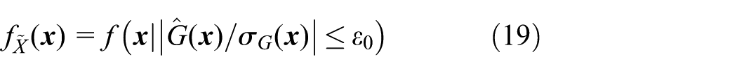
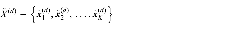
• Step 1. For the Kriging model already constructed, generate K random points on or almost on $\hat{G}(\mathit{x})=0$ . They are treated as the candidates of the representative points to refresh the current DoE. It is theoretically impossible that samples from random simulation method are exactly located on $\hat{G}(\mathit{x})=0$ . Hence, the less-than-ideal alternative is to make them satisfy equation (18)

$$\left|\frac{\hat{G}(\mathit{x})}{{\sigma }_G(\mathit{x})}\right|\le {\epsilon }_0$$

(18)

where ε₀ > 0. The lower ε₀ is, the closer x is to $\hat{G}(\mathit{x})=0$ . This article sets ε₀ = 0.1, as $\Phi (-0.05)\approx 0.46$ . Let $\tilde{X}$ denotes the i.i.d. point set as well as the candidate set of the representative points mentioned above

$$\tilde{X}=\{{\tilde{\mathit{x}}}_1,{\tilde{\mathit{x}}}_2,\dots ,{\tilde{\mathit{x}}}_K\}$$

Both MCS and Markov chain Monte Carlo (MCMC) are suitable to generate $\tilde{X}$ . And the latter is adopted here. The conditional PDF for generating $\tilde{X}$ is

$$f_{\tilde{X}}(\mathit{x})=f(\mathit{x}||\hat{G}(\mathit{x})/{\sigma }_G(\mathit{x})|\le {\epsilon }_0)$$

(19)

The domain defined by equation (18) is very cabined. It is almost sure that its proportion in the whole X space is below that of the estimated failure domain, that is, the estimate of the failure probability

$$\underset{|\hat{G}(\mathit{x})/{\sigma }_G(\mathit{x})|\le {\epsilon }_0}{\int }f(\mathit{x})\mathrm{d}\mathit{x}<\underset{\hat{G}(\mathit{x})\le 0}{\int }f(\mathit{x})\mathrm{d}\mathit{x}$$

(20)

According to equation (13), the coefficient of variation of ${\hat{P}}_f$ approximates to $1/\sqrt{N_{\mathrm{MC}}{\hat{P}}_f}$ . In another word, $1/\sqrt{N_{\mathrm{MC}}{\hat{P}}_f}$ ( $N_{\mathrm{MC}}{\hat{P}}_f$ , the number of the random samples located in $\hat{G}(\mathit{x})\le 0$ ) is available to measure how well the dispersion of the estimated failure samples is. Similarly, this article employs $1/\sqrt{K}$ to measure the dispersion of the i.i.d. points in the vicinity of $\hat{G}(\mathit{x})=0$

$$K\to \infty \Rightarrow 1/\sqrt{K}\to 0$$

As $N_{\mathrm{MC}}{\hat{P}}_{\mathrm{f}}=3\times {10}^3$ ( ${\delta }_{\mathrm{MC}}\approx 0.018$ ) is enough for most of the engineering problems, this article proposes K = 3 × 10³ ∼ 10⁴.

• Step 2. Reduce the dimension of points in $\tilde{X}$ from M to d (d < M) with Isomap technique. $\tilde{X}$ is mapped to a d-dimension point set ${\tilde{X}}^{(d)}$

$${\tilde{X}}^{(d)}=\{{\tilde{\mathit{x}}}_1^{(d)},{\tilde{\mathit{x}}}_2^{(d)},\dots ,{\tilde{\mathit{x}}}_K^{(d)}\}$$

where ${\tilde{\mathit{x}}}_i^{(d)}$ is corresponding to ${\tilde{\mathit{x}}}_i$ in $\tilde{X}$ (i = 1, 2, …, K). Isomap is used to straighten the “curve” $|\hat{G}(\mathit{x})/{\sigma }_G(\mathit{x})|\le {\epsilon }_0$ (M = 2) and spread out the “surface” (M = 3) or the “hyper-surface” (M > 3). This article sets d = M–1 for simplification (determining the optimal d during dimensionality reduction is a complicated problem).

• Step 3. Pick k representative points in $\tilde{X}$ . Group ${\tilde{X}}^{(d)}$ into k clusters by clustering algorithm and get k centers ${\mathit{\mu }}_i^{(d)}$ (i = 1, …, k). In $\tilde{X}$ , approximate inverse images of ${\mathit{\mu }}_i^{(d)}$ (i = 1, …, k) are the representative points mentioned above.

Step 2 and step 3 are illustrated in detail in sections “Framework of MSFA–SVR” and “Pre-adaptation results integration.”

According to equations (18) and (19), the area where points are with larger values of $f_{\tilde{X}}(\mathit{x})$ (which is proportional to f( x ) and quantifies the importance of x to P_f) and ${\sigma }_G(\mathit{x})$ (which measures the epistemic uncertainty of G( x )) tends to gather more random points. Therefore, the representative points are more likely to locate in the area(s) of interest, as a result of which the Kriging model could be directly improved.

Dimensionality reduction of $\tilde{X}$ with Isomap

Isomap is one of the most widely applied nonlinear dimensionality reduction techniques. It performs low-dimensional embedding based on the geodesic distance which is the sum of edges along the shortest path between points. The main steps of Isomap algorithm are summarized as follows:

• Step 1. Define neighbor set of each point. The neighbor set of ${\tilde{\mathit{x}}}_i$ in $\tilde{X}$ consists of its $n_{\mathit{x}}$ nearest neighbors.

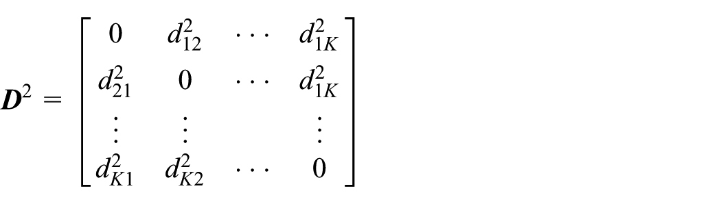
• Step 2. Construct the neighborhood graph over all points and compute the pairwise geodesic distance to get the squared geodesic distance matrix D ² . Geodesic distance is the sum of edge length which is equal to the Euclidean distance along the shortest path between points

$${\mathit{D}}^2=\left[\begin{array}{cccc}0\hfill & d_{12}^2\hfill & ···\hfill & d_{1K}^2\hfill \\ \multicolumn{1}{c}{d_{21}^2}& 0\hfill & ···\hfill & d_{1K}^2\hfill \\ \multicolumn{1}{c}{⋮}& ⋮\hfill & \hfill & ⋮\hfill \\ \multicolumn{1}{c}{d_{K1}^2}& d_{K2}^2\hfill & ···\hfill & 0\hfill \end{array}\right]$$

where $d_{\mathrm{ij}}$ is the geodesic distance between ${\tilde{\mathit{x}}}_i$ and ${\tilde{\mathit{x}}}_j$ in $\tilde{X}$ .

• Step 3. Perform lower dimensional embedding by applying multidimensional scaling to the acquired pairwise geodesic distances and get the d-dimension point set ${\tilde{X}}^{(d)}$

$$s_i^p=\sqrt{{\lambda }_p}{v}_p^i,i=1,\dots ,K;p=1,\dots ,d$$

(21)

$$\begin{array}{c}\mathit{Q}=\frac{1}{2}\mathit{H}{\mathit{D}}^2\mathit{H}\hfill \\ \mathit{H}={\mathit{I}}_K-\frac{1}{K}{\mathit{e}}_K{\mathit{e}}_K^{\mathrm{T}}\hfill \\ {\mathit{e}}_K=[1,1,\dots ,1{]}^{\mathrm{T}}\in R^K\hfill \end{array}$$

where ${\lambda }_p$ is the pth eigenvalue of matrix Q and ${\mathit{v}}_p$ is the corresponding eigenvector of ${\lambda }_p$ .

Cluster analysis with k-means clustering algorithm

k-means clustering is a cluster analysis method whose aim is to group a set of objects into several clusters while guaranteeing that the objects in the same cluster are more similar to each other than to those in any other clusters. Given the point set ${\tilde{X}}^{(d)}$ , k-means clustering groups ${\tilde{X}}^{(d)}$ into k clusters $\{{\tilde{X}}_1^{(d)},{\tilde{X}}_2^{(d)},\dots ,{\tilde{X}}_k^{(d)}\}$ so as to minimize the within-cluster sum of squares (WCSS)

$$\underset{{\tilde{X}}^{(d)}}{\arg min}\sum _{i=1}^k\sum _{{\mathit{x}}^d\in {{\tilde{X}}_i^{(d)}}_i}||{\mathit{x}}^d-{\mathit{\mu }}_i^{(d)}|{|}^2$$

(22)

where ${\mathit{\mu }}_i^{(d)}$ is the mean of points in ${\tilde{X}}_i^{(d)}$ . The M-dimension point corresponding with ${\mathit{\mu }}_i^{(d)}$ is not unique because of d < M. Moreover, as the iterative procedure goes and $\hat{G}(\mathit{x})=0$ converges to G( x ) = 0 gradually, representative points may be too close to some points in current DoE and result in ill-condition design matrix ( G in equation (6)) and worse quality of DoE points. To overcome the awkward situations, the representative points of $\tilde{X}$ are acquired according to equations (23) and (24)

$${\tilde{\mathit{x}}}_{I_i}=\underset{\tilde{\mathit{x}}\in \tilde{X}}{\arg min}||{\tilde{\mathit{x}}}^{(d)}-{\mathit{\mu }}_i^{(d)}|{|}^2(i=1,\dots ,k)$$

(23)

$$\{\begin{array}{c}||\tilde{\mathit{x}}-{\mathit{x}}_n||\ge d_{0}n=1,\dots ,N\mathrm{and}{\mathit{x}}_n\in {\mathit{S}}_{\mathrm{DoE}}\hfill \\ \multicolumn{1}{c}{||\tilde{\mathit{x}}-{\tilde{\mathit{x}}}_{I_j}||\ge d_{0}j=1,\dots ,i-1}\end{array}$$

(24)

whereas in this article

$$d_0=0.9min\{||{\mathit{x}}_m-{\mathit{x}}_n||;m\ne n,{\mathit{x}}_m,{\mathit{x}}_n\in {\mathit{S}}_{\mathrm{DoE}}\}$$

The proposed reliability analysis method

This section constructs an adaptive structural reliability analysis method, which is mainly based on the proposed Isomap-Clustering strategy in section “Specification on proposed method.” In the proposed method, the surrogate model of the performance function is based on the sparse polynomial-Kriging illustrated in section 2, and the proposed Isomap-Clustering strategy in section “Specification on proposed method” is employed to iteratively improve the Kriging model until its accuracy meets the stopping criterion defined by derivation. The main steps of the adaptive method are listed as follows:

• Step 1. t = 0. Generate the initial DoE with Latin hypercube sampling (LHS) and call to the performance function to calculate the performance values at the initial DoE points. The hyper-rectangle of LHS is [−nσ, nσ] ^M , and the initial number of points is N₀. This article sets n_σ = 5

$$\begin{array}{c}{\mathit{S}}_{\mathrm{DoE}}=[{\mathit{x}}_1,{\mathit{x}}_2,\dots ,{\mathit{x}}_{N_0}]\hfill \\ \mathit{Y}=[y_1,y_2,\dots ,y_{N_0}{]}^T\hfill \end{array}$$

• Step 2. Construct the Kriging model ${\hat{G}}_t(\mathit{x})$ and ${\sigma }_G^2(\mathit{x})$ based on sparse polynomial-Kriging and compute the estimated failure probability ( ${\hat{P}}_{f,t}$ ). Section “Research background” details the theory of the Kriging model and method for selecting the basic function with LAR and AIC. The integral of equation (11) is approximately performed with MCS, and ${\tilde{P}}_{f,t}$ denotes the estimation of ${\hat{P}}_{f,t}$

$${\tilde{P}}_{\mathrm{f},t}=\frac{1}{N_{\mathrm{MC},t}}\sum _{i=1}^{N_{\mathrm{MC},t}}{I}_{{\hat{G}}_t<0}\left({\mathit{x}}_{\mathrm{MC},i}\right)$$

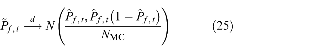
According to the central limit theorems, ${\tilde{P}}_{f,t}$ converges in distribution to a normal distribution

$${\tilde{P}}_{f,t}\stackrel{d}{\to }N\left(\frac{{\hat{P}}_{f,t},{\hat{P}}_{f,t}(1-{\hat{P}}_{f,t})}{N_{\mathrm{MC}}}\right)$$

(25)

Then

$$\begin{array}{l}P\left(|{\tilde{P}}_{\mathrm{f},t}-{\widehat{P}}_{\mathrm{f},t}|<e{\widehat{P}}_{\mathrm{f},t}\right)\approx 2\Phi (e{\widehat{P}}_{\mathrm{f},t}\sqrt{\frac{N_{\mathrm{MC},t}}{{\widehat{P}}_{\mathrm{f},t}(1-{\widehat{P}}_{\mathrm{f},t})}})\\ -1\approx 2\Phi (e\sqrt{{\widehat{P}}_{\mathrm{f},t}{N}_{\mathrm{MC},t}})-1\end{array}$$

(26)

where e > 0. $\Phi (·)$ is the cumulative distribution function (CDF) of the standard normal distribution. The failure probability is generally with small magnitude, so $1-{\hat{P}}_{\mathrm{f},t}$ in the denominator is neglectable. It is set that the relative error of ${\tilde{P}}_{\mathrm{f},t}$ is no larger than 3% with confidence level 0.95

$$P(|{\tilde{P}}_{\mathrm{f},t}-{\hat{P}}_{\mathrm{f},t}|<0.03{\hat{P}}_{\mathrm{f},t})\ge 0.95$$

According to equation (26)

$$2\Phi (0.03\sqrt{{\hat{P}}_{\mathrm{f},t}{N}_{\mathrm{MC},t}})-1\ge 0.95$$

Then

$$N_{\mathrm{MC},t}{\hat{P}}_{\mathrm{f},t}\ge 4268$$

(27)

$N_{\mathrm{MC},t}{\hat{P}}_{\mathrm{f},t}$ is the expectation of failure number among $N_{\mathrm{MC},t}$ random samples, so this article sets that MCS terminates until the number of failure random samples is above 4300.

• Step 3. Judge whether the iterative procedure is convergent. If ${\tilde{P}}_{\mathrm{f},t}$ and ${\tilde{P}}_{\mathrm{f},t-1}$ satisfy equation (28), terminate the procedure. ${\tilde{P}}_{\mathrm{f},t}$ is the estimate of the target failure probability. Otherwise, continue and go to step 4.

When both ${\hat{G}}_{t-1}(\mathit{x})=0$ and ${\hat{G}}_t(\mathit{x})=0$ , approximate G( x ) = 0 well enough, and they satisfy that

$$\begin{array}{c}{N}_{\mathrm{MC},t}\approx N_{\mathrm{MC},t-1}\to N_{\mathrm{MC}}\hfill \\ {\hat{P}}_{f,t}\approx {\hat{P}}_{f,t-1}\to {\hat{P}}_f\hfill \end{array}$$

Taking equation (25) into consideration,

$$P(\frac{{\tilde{P}}_{f,t}-{\tilde{P}}_{f,t-1}}{{\hat{P}}_f}\le 1.96\sqrt{\frac{2(1-{\hat{P}}_f)}{{\hat{P}}_f{N}_{\mathrm{MC}}}})\approx 0.95$$

According to equation (27)

$$P(\frac{{\tilde{P}}_{f,t}-{\tilde{P}}_{f,t-1}}{{\hat{P}}_f}\le 0.0424)\approx 0.95$$

Therefore, the reliability analysis procedure is regarded as convergent if the relative error between ${\tilde{P}}_{f,t}$ and ${\tilde{P}}_{f,t-1}$ is less than 4%

$$\frac{{\tilde{P}}_{f,t}-{\tilde{P}}_{f,t-1}}{\left({\tilde{P}}_{f,t}+{\tilde{P}}_{f,t-1}\right)/2}\le 4\%$$

(28)

• Step 4. t = t + 1. Carry out the Isomap-Clustering strategy and refresh the current DoE. Search the representative points in the vicinity of ${\hat{G}}_{t-1}(\mathit{x})=0$ by employing the Isomap-clustering strategy proposed in section “Research background” and compute their performance function values. Refresh the current DoE and Y and return to step 2.

Numerical applications

In this section, three examples are analyzed to demonstrate the advantage of the proposed Isomap-Clustering strategy. Two of them have explicit performance functions and the other one is implicit.

Example 1: an analytical example with two input variables

The first analytical example with two input variables has already been analyzed in Roussouly et al. ³³ It is adopted here to visualize the Isomap-Clustering strategy. The performance function is

$$G(\mathit{x})=\exp (0.4x_1+7)-\exp (0.3x_2+5)-200$$

where X  = [X₁, X₂]^T subjects to standard bivariate normal distribution and X₁ and X₂ are mutually independent. The failure domain G( x ) ≤ 0 is equivalent to

$$x_1\le 2.5[\ln (\exp (0.3x_2+5)+200)-7]$$

The target failure probability is

$$\begin{array}{l}{P}_{\mathrm{f}}=\frac{1}{2\pi }{\displaystyle \underset{-\infty }{\overset{+\infty }{\int }}\exp (-x_2^2/2)·\left({\displaystyle \underset{-\infty }{\overset{u(x_2)}{\int }}\exp (-x_2^2/2)\mathrm{d}{x}_1}\right)}\\ \mathrm{d}{x}_2\approx 3.62\times {10}^{-3}\end{array}$$

(29)

where

$$u(x_2)=2.5[\ln (\exp (0.3x_2+5)+200)-7]$$

According to equation (30), the target reliability index ( $\beta$ ) is 2.686

$$\beta =-{\Phi }^{-1}\left(P_f\right)$$

(30)

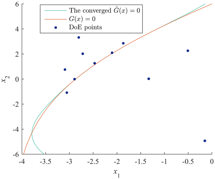
The method constructed in section “The proposed reliability analysis method” is applied to this example with N₀ = 6, K = 300, and k = 3. The proposed reliability analysis method based on Isomap-Clustering strategy satisfies the stopping criterion defined by equation (28) when t = 3. Figure 2 visualizes the DoE points from the Isomap-Clustering and the Kriging-based $\widehat{G}(\mathit{x})=0$ of each iteration. Figure 3 compares the convergent $\hat{G}(\mathit{x})=0$ and G(x) = 0 and shows the DoE points to construct the convergent Kriging model. Figures 2 and 3 demonstrate that most of the DoE points from Isomap-Clustering strategy are located in area of interest and that the concentration of DoE points is successfully avoided. Results are summarized in Table 1.

Figure 2.

The process of iterations for example 1. Subfigure (a), (b) and (c) correspond with the 1st, 2nd and 3rd iteratives of the proposed method, respectively. The legend shown in subfigure (a) is also valid for subfigure (b) and (c).

Figure 3.

The comparison between the convergent $\hat{G}(\mathit{x})=0$ and G( x ) = 0.

Table 1.

Results of example 1.

$P_{\mathrm{f}}$	${\hat{P}}_{\mathrm{f}}$	$\beta$	$\hat{\beta }$	N call
3.62 × 10−3	3.63 × 10−3	2.686	2.685	15

Example 2: an analytical example with six input variables

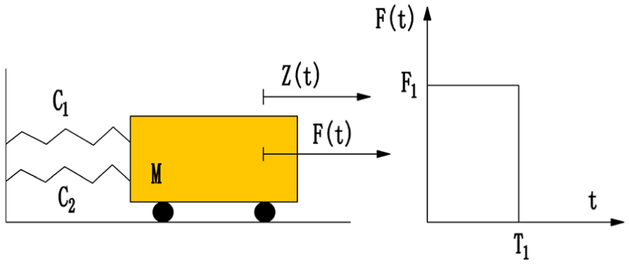
The second analytical example with six input variables handles the nonlinear undamped single degree of freedom system shown in Figure 4. It has already been studied in literatures.^13,17,34 Its performance function is defined as

$$g(C_1,C_2,M,R,T_1,F_1)=3R-\left|\frac{2F_1}{M{\omega }_0^2}\sin \left(\frac{{\omega }_0{T}_1}{2}\right)\right|$$

(31)

where

$${\omega }_0=\sqrt{(C_1+C_2)/M}$$

Figure 4.

The nonlinear undamped single-degree-of-freedom system.

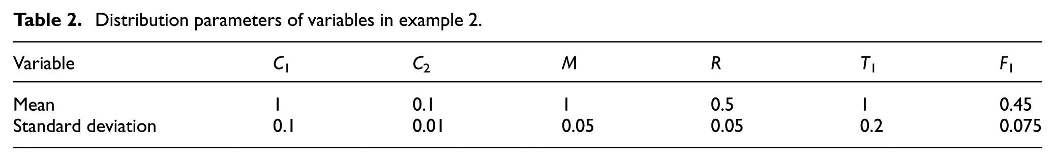
All input variables are mutually independent and subject to normal distribution. Their means and standard deviations are listed in Table 2. The referential failure probability obtained from MCS with 10⁶ simulations is 2.87 × 10⁻².

Table 2.

Distribution parameters of variables in example 2.

Variable	C 1	C 2	M	R	T 1	F 1
Mean	1	0.1	1	0.5	1	0.45
Standard deviation	0.1	0.01	0.05	0.05	0.2	0.075

First, all inputs are transformed to the standard normal distribution according to equation (32). To investigate the influence of k on efficiency of the Isomap-Clustering strategy, the reliability analysis method proposed in section “Empirical comparison and discussion” is run five times with N₀ = 10, K = 3000, and different values of k (k = 4, 5, 6, 7, 8)

$$x~N(\mu ,{\sigma }^2)\iff \frac{x-u}{\sigma }~N(0,1)$$

(32)

Results from the proposed method and AK-MCS-based methods are summarized in Table 3. N_call, ${\hat{P}}_f$ , δ, and ε_% listed in Table 3 stand for the number of calls to the performance function (equation (31)), the estimate of the target failure probability, the coefficient of variation of ${\hat{P}}_f$ , and the relative error of ${\hat{P}}_f$ compared with the reference value, respectively. According to Table 3, it seems that k affects N_call of the proposed method slightly. With acceptable accuracy (ε_%), the number of calls to performance function (N_call) is lower than other methods listed in Table 3. Moreover, the iterations of the proposed method is much fewer than the Kriging-based methods AK-MCS+U and AK-MCS+EFF because the Isomap-Clustering strategy refreshes the Kriging model with a few points, while they do it with only one point each iteration.

Table 3.

Comparisons of results of example 2.

Method	N call	Iterations	${\hat{P}}_f$ (10−2)	δ (%)	ε (%)
MCS	106	–	2.87	0.59	–
AK-MCS + U	57	47	2.85	1.85	<0.1
AK-MCS + EFF	55	45	2.86	1.80	0.39
The proposed method	46 (k = 4)	9	2.85	0.67	0.63
	40 (k = 5)	6	2.87	0.67	<0.1
	40 (k = 6)	5	2.84	0.66	0.58
	38 (k = 7)	4	2.85	0.65	0.61
	42 (k = 8)	4	2.86	0.68	0.29

MCS: Monte Carlo simulation; EFF: expected feasibility function.

Example 3: truss structure with 10 dimensions

This truss structure has already been studied in Roussouly et al. ³³ and Blatman and Sudret. ³⁵ As shown in Figure 5, it contains 11 horizontal bars and 12 sloping ones. A₁ and E₁ denote horizontal bar’s cross section and Young’s moduli, respectively, while A₂ and E₂ denote sloping bars: six loads, from P₁ to P₆, are applied on nodes of horizontal bars. These 10 random variables are independent of each other, and their distribution information is listed in Table 4.

Figure 5.

The truss structure (unit meter).

Table 4.

Distribution information of variables in example 2.

Variable	Distribution	Mean	Standard deviation
P 1–P6	Gumbel	$5\times {10}^4$	$7.5\times {10}^3$
A 1	Lognormal	$2\times {10}^{-3}$	$2\times {10}^{-4}$
A 2	Lognormal	$1\times {10}^{-3}$	$1\times {10}^{-4}$
E 1	Lognormal	$2.1\times {10}^{11}$	$2.1\times {10}^{10}$
E 2	Lognormal	$2.1\times {10}^{11}$	$2.1\times {10}^{10}$

The deflection of node 1 in Figure 5 denoted by s ( x ) is the response of the structure. The threshold of | s ( x )| is 0.14m in accordance with Roussouly et al. ³³ The performance function of the truss structure is

$$G(\mathit{x})=0.14-|\mathit{s}(\mathit{x})|$$

According to Roussouly et al. ³³ and Blatman and Sudret, ³⁵ the referential failure probability ( $P_f^{\mathrm{REF}}$ ) and reliability index ( ${\beta }^{\mathrm{REF}}$ ) are $3.45\times {10}^{-5}$ and 3.98, respectively, which is from IS with 500,000 simulations.

After transforming the variables in Table 4 to the standard normal distribution, apply the proposed method to the truss structure 10 times with N₀ = 15, K = 3000, and different values of k (k = 4, 5, 6, 7, 8) to test its stability. Results are summarized in Table 5. Figure 6 shows the convergent process of ${\hat{P}}_f$ and $\hat{\beta }$ . The stopping criterion proposed in Tong et al. ¹⁹ is employed as the condition of convergence of AK-MCS-based methods, as the one proposed in Echard et al. ¹⁷ , is apparently too rigorous and equation (28) is not available for AK-MCS.

Table 5.

Comparisons of results of example 3.

Method	N call	Iterations	${\hat{P}}_f$ (10−5)	δ (%)	$\hat{\beta }$
IS	5 × 105	−	3.45	1.5	3.98
AK-MCS + U	145	130	3.35	1.51	3.99
AK-MCS + EFF	160	145	3.33	1.53	3.99
The proposed method	115 (k = 4)	25	3.39	1.51	3.98
	107 (k = 4)	23	3.44	1.45	3.98
	120 (k = 5)	21	3.32	1.47	3.99
	115 (k = 5)	20	3.31	1.50	3.99
	105 (k = 6)	15	3.40	1.49	3.99
	117 (k = 6)	17	3.32	1.50	3.99
	99 (k = 7)	12	3.30	1.47	3.99
	106 (k = 7)	13	3.36	1.50	3.99
	111 (k = 8)	12	3.35	1.48	3.99
	103 (k = 8)	11	3.38	1.49	3.98

MCS: Monte Carlo simulation; EFF: expected feasibility function.

Figure 6.

The convergence procedure of ${\hat{P}}_f$ and $\hat{\beta }$ . AK-MCS+EFF means that the corresponding results (i.e. the estimates of the targer failure probability and reliability index) are from AK-MCS+EFF, and other lines are in a similar way. Subfigures (a) and (c) correspond to subfigures (b) and (d), respectively. All the subfigures share the legend shown in subfigure (a).

Conclusion

This article proposes an innovative DoE strategy for Kriging-based reliability analysis method. The strategy, named as Isomap-Clustering strategy, is able to refresh the Kriging model with several representative points in the vicinity of the estimate of the limit state each iteration. In the innovative strategy, Isomap method andk-means clustering algorithm are employed to determine the representative points among hundreds, even thousands, of candidates. A Kriging-based active reliability analysis method which employs sparse polynomial-Kriging model and Isomap-Clustering strategy is also constructed. As a modification of original Kriging model, sparse polynomial-Kriging is more flexible in terms of basic regression function. To validate the proposed DoE strategy and the reliability method, three examples are analyzed. From the results, the following can be concluded:

1. Most of the Isomap-Clustering strategy–based points to refresh DoE and the Kriging model are well-proportioned located in the area of importance to the accuracy of the estimate of failure probability, which makes the Kriging model efficiently improved and the Kriging-based estimate of failure probability convergent with calling to the performance function fewer times.

2. As the DoE of the Kriging model is refreshed by a few points each iteration, the proposed Isomap-Clustering strategy is able to remarkably reduce the iterative times of Kriging-based reliability analysis method. By employing parallel computing or distributed computing, the efficiency of structural reliability analysis with time-consuming performance function is surely enhanced.

3. According to the results of the second and third examples, the efficiency of Isomap-Clustering strategy is not sensitive to the number of the representative points (k in equation (22)) in the vicinity of the Kriging-based $\hat{G}(\mathit{x})=0$ , which means that k could be determined mainly according to the parallelizability capacity.

The basic idea of the proposed strategy is to refresh the Kriging model with a few representative points in the vicinity of $\hat{G}(\mathit{x})=0$ , and Isomap technique and k-means clustering algorithm are used to achieve the goal. Theoretically, the efficiency of the Isomap-Clustering strategy suffers no loss if generating more random candidates of the representative points. Besides, increasing the number of the initial DoE points apparently benefits the initial Kriging model as well as the iterative times of reliability analysis. Therefore, both values (K and N₀) are not discussed in section “Conclusion.” Different Kriging-based methods are fairly compared with the same values of N₀. The performance function of the third example is implicit, which often occurs in engineering. As numerical model of structures in engineering becomes more and more time-consuming, minimizing the number of calls to performance function and iterations directly reduce the time cost of reliability analysis. The success of the proposed method in the third example demonstrates its potential to engineering applications.

As Isomap is a wonderful method to map points on a hyperplane into lower dimension, the proposed Isomap-Clustering strategy may be not suitable for reliability analysis problems with more than one failure sub-domain.