
Abstract
A brake-by-wire system is considered the best solution to realize advanced functions in electric vehicles/hybrid electric vehicles and intelligent vehicles. In this article, a novel electro-hydraulic brake system is proposed. The main issues in the development of the proposed electro-hydraulic brake system focus on hydraulic loop design and pressure tracking control. Instead of an accumulator, a large displacement piston pump coupled to a high-power motor is applied to meet the demand of pressure boost. A passive pedal feel simulator is designed to decouple the brake pedal and the wheel cylinders. The high pressure in the wheel cylinders is controlled by de/activating the motor and valves to track the reference pressure. To minimize the pressure instability observed in previous proportional–integral–derivative controller tests, a self-tuning generalized predictive controller is applied. Models of each system’s dynamic process are derived, and the parameters are identified through test data. A sliding mode differentiator is used to filter the sensor signals and improve the pressure boost performance in hard brake maneuvers. A rapid control prototype test environment based on dSPACE is built to verify and adjust the controller. The simulation results using MATLAB/Simulink and bench tests are presented and analyzed. Tracking performances show that compared to a proportional–integral–derivative controller, the proposed controller has a better effect in lowering pressure overshoots and start–stop frequency.
Keywords
Introduction
Brake-by-wire (BBW) systems have the inherent advantages of being small in size and flexible for brake force control. When the pedal feel simulator (PFS) decouples the drivers’ feet and the wheels, BBW systems precisely manage the brake force of each wheel without disturbing the pedal feel. With the development of hybrid electric vehicles (HEVs), electric vehicles (EVs), and intelligent vehicles, brake systems are required to offer advanced functions, such as regenerative braking (RB), active safety, and autonomous drive; BBW systems are widely considered the best option to meet these demands.
Generally, BBW systems are classified into two groups: electro-hydraulic brake (EHB) and electro-mechanical brake (EMB) systems. Compared with EMB, EHB systems have a simpler structure and smoother pressure transmission. In support of current motor and valve technologies, EHB could have a comparatively low development period and provide profits more quickly. 1
The electronically controlled brake (ECB®) by Advics is the earliest EHB production case; it was initially developed for the Toyota Prius and Lexus hybrid models. 2 Around the same time, Daimler–Benz implemented another EHB, the sensotronic brake control (SBC®) by Bosch, into its W211, R230, and W219 models. 3 However, this type of EHB did not appear in the next generation of Benz models because of reliability considerations. In recent years, auto part suppliers have invented ball-screw (or worm-gear) EHBs. Typical prototypes include iBooster® by Bosch, MK-C1® by Continental Teves, IBC® by ZF-TRW, and ESB® by Honda. Among these prototypes, ESB is already in small-scale production and has been used to coordinate with Honda’s HYBRID SH-AWD technique in some high-performance models, such as the NSX and MK-C1, and it has been implemented in Alfa Romeo models.
However, the market share of EHB has not obviously increased in the past decade. Instead, the electric vacuum pump (EVP) solution has been widely applied in current EV/HEVs. Although EHB has a huge marketing potential, currently, the cost, reliability, and brake force control difficulty impede its development.
In Reuter et al., 4 the authors compared Delphi’s EHB with conventional vacuum-booster brake systems and highlighted various valuable design options. In Velardocchia, 5 a methodology based on hardware-in-loop (HIL) was illustrated to evaluate the dynamic characteristics of EHB components. Beyond these examples, the works of many other researchers have inspired our team to design a low-cost EHB. Different from the cylinder volume-change concept of ball-screw (or worm-gear) EHBs, the flow-change concept is adopted in our proposed EHB configuration. An analogous concept was used in an autonomous vehicle application. 6 In our proposed EHB, no volume recovery time (turn back screw) and infinite fluid flow in the loop could provide continuous and stable pressurization.
Non-model proportional–integral–derivative (PID) controllers have been adopted to address pressure tracking issues in many similar studies, whereby simulations and HIL tests have verified the effectiveness of the controllers.7,8 Those results, although attractive, had deficiencies in that the simulations and bench tests did not consider humidity, pad wearing and temperature, and other uncertain factors. In fact, variation of parameters is the main cause of delay and poor control accuracy. Because of the feedback structure of normal PIDs, the effects of controller outputs always fall behind the delays, including hydraulic delay, electro-mechanical delay, signal transmitting, and processing delay. Larger overshoots lead to increases in both adjustment times and energy consumption. There is still a demand for improving the pressure control precision. In Todeschini et al., 9 a hybrid control based on a position-pressure map was described to address the huge overshoot caused by dead-zone delay. In Line et al., 10 predictive control was used to improve the utilization of motor torque in EMB force control. In particular, in the proposed EHB, when the motor began to work, the rotor would remain statically until the increasing current overcame the friction in the piston. This effect leads to a slightly longer time delay compared to that of other EHBs. To achieve a balance in rapidity and accuracy, in this article, a generalized predictive control (GPC) method is adopted to optimize the pressure tracking performance. GPC is suitable for this EHB system because (1) it has complete theoretical support for linear single input single output systems and effective means to solve the objective min J with variable constraints; (2) it is able to estimate future system responses and compute the corresponding future controller outputs to eliminate the overshoots caused by the delay; (3) in this study, the GPC controller uses the extended auto-regressive (ARX) model, which contains delay and disturbance, and can be feasibly identified and self-tuned online. 11
The rest of paper is organized as follows. In section “System descriptions,” we outline the design concept of the proposed EHB system and the rapid control prototype (RCP) test environment. In section “System modeling and identification,” the dynamic models of the pressurizing and depressurizing stages are derived and identified. In section “Pedal movement,” we propose a methodology based on the Levant differentiator (LD) to filter signals and realize the brake assist (BA) function. In section “Controller design,” self-tuning GPC laws are designed to improve the pressure tracking performance under simulation. The proposed controller is experimentally validated in section “Test verification of the pressure tracking,” and our final conclusions are given in section “Conclusion.”
System descriptions
Hydraulic loop design
Figure 1 shows the self-designed prototype. The components, such as the motor pump, valves, and main cylinder, were integrated into one block. A schematic portrait of the overall system is shown in Figure 2. Under normal brake situations, the system is pressurized by a high-power direct current (DC) motor coupling with a large displacement pump and depressurized by the high-speed on/off solenoid reducing valve 6. When the electrical supply is operating, the normally closed valves 1, 3, and 5 are opened, whereas the normally open valves 2 and 4 are closed; as a result, the PFS decouples the low-pressure main cylinder and the high-pressure wheel cylinders. An angle sensor detects the pedal movements and provides a reference wheel pressure for the controller. Pressure sensors located at the wheel cylinders provide feedback signals to the controller. When the electrical supply fails, an alternative hydraulic loop ensures the emergency brake is engaged. By depressing the brake pedal, brake fluid is still able to flow into the wheel cylinders through the main cylinder and valves 2 and 4.
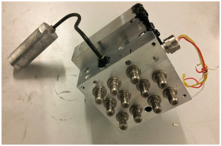
HCU and PFS prototype.

Configuration diagram of the EHB system.
An apparent difference between the proposed EHB system and other EHB systems is that the proposed system has no accumulator. In accumulator-type EHBs, the life of the accumulator is a main factor limiting reliability. Instead, in the proposed EHB system, a high-power DC motor (500 W with a 12-V supply) and a four-piston pump are self-designed to meet the pressure boost requirements, that is, a controller is required to determine the motor speed and start/stop timing. Similar to anti-lock brake system (ABS), there are two valves for each wheel to regulate the pressure individually. As shown in Figure 3, the vector of the target reference pressure is determined by many factors. The vector contains a comprehensive set of logical operation functions, such as brake pedal movements, electronic brakeforce distribution/Electronic stability control (EBD/ESC), adaptive cruise control (ACC), and RB. In production vehicles, the reference pressure is provided by a vehicle control unit (VCU). The complete algorithm will not be analyzed here. In this article, we focus on the precise pressure control under normal braking situations, that is, the reference pressure is calculated based only on the brake pedal angle sensor signals.

Operation block diagram of the EHB system.
RCP test environment
An RCP test environment was designed to achieve system identification and control algorithm verification. Figure 4 shows the structural diagram of the test environment. For the software, Controldesk® serves as a bridge connecting MATLAB and dSPACE Autobox and provides configuration functions, including display, recording, signal transmission, and interface design. Control algorithms are designed in Simulink and then programmed into dSPACE. One angle sensor and four pressure sensors are responsible for signal acquisition. The pulse width modulation (PWM) generator integrated in dSPACE and a circuit board drive the actuators of the EHB. Depending on different experimental purposes, the test modes can be switched between open-loop and closed-loop configurations.
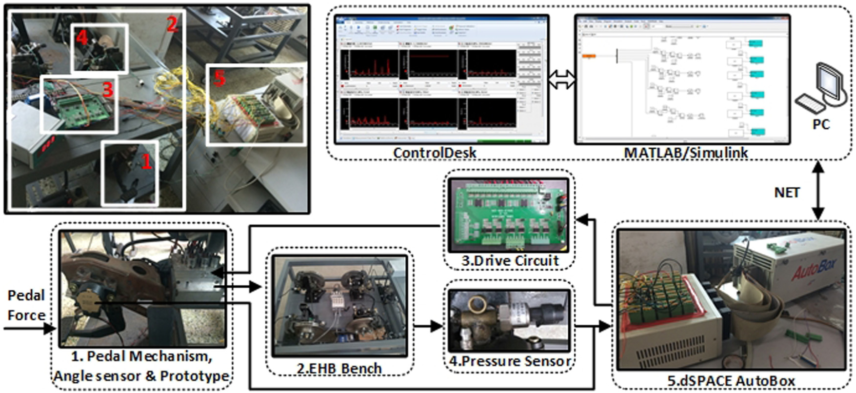
RCP test environment.
System modeling and identification
GPC controllers are based on reference models. In this section, the model of each dynamic stage is discussed and identified.
Subsystem models
When there is no brake pressure distribution activation or proportional valve, the pump pushes the fluid into the four wheel cylinders. Because the motor and the valve have different control intervals (see the later discussion), for convenience, we use a continuous model to describe the dynamic processes in each subsystem and then separately study each controller of the pressurization and depressurization stages through discrete models. The dynamic equations of each subsystem during the pressurization process are as follows:
Motor

Pump

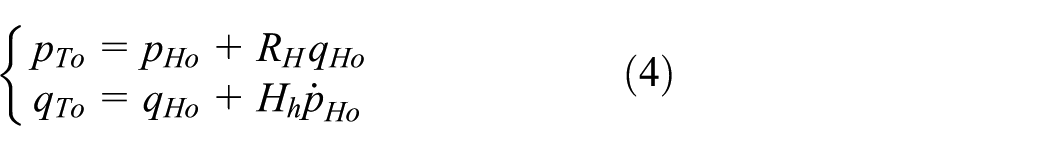
Brake tube

Brake hose
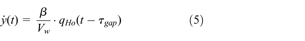
Wheel cylinder
where, in equation (1),
A high-speed on/off valve, labeled valve 6, is used for depressurizing at 50 Hz, which is an appropriate carrier frequency. The average flow rate of fluid

where
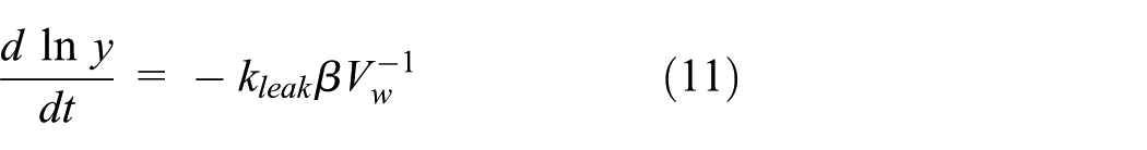
Leakage generally exists in high-pressure hydraulic systems. A leakage model should be considered when the system model must accurately simulate real hardware and when a controller is required for better accuracy and robustness. Assuming that there are no leakages from the interior of the hydraulic circuit to the exterior, the total quantity of brake fluid in the system remains unchanged. The leakages occur at the orifices, where a large pressure difference exists between the inlet and the outlet. From equation (2), the flow rate of system leakage

Equation can be log-linearized to

System identification
Nonlinear input separation
For a motor pump, there is a memoryless static nonlinear relationship between the actual drive voltage and the output speed corresponding to the inherent load force of friction and the spring in the pump. When the rotor is driven, it does not rotate immediately until the rising current overcomes the load force; as a result, the proposed EHB has a larger delay than accumulator-type EHBs. Similarly, for a valve, both the dead-zone and saturation-zone nonlinear input exist. At small and large PWM inputs, there are nearly no changes in the fluid flow rates. Several tests were performed to estimate the static nonlinear properties; some typical data are shown in Figure 5. As seen in Figure 5(a), when the actual driven PWM input was lower than approximately 0.3, the motor pump did not operate. Moreover, in Figure 5(b), the effective operation range of the valve was narrower, and the flows for large or small driven inputs were almost identical. If we take the initial slope values of the curves as fit points, then we have the approximate static nonlinear properties of two inputs, as shown in Figure 6.
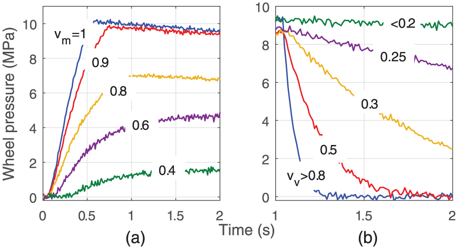
Pressure responses of different drive inputs: (a) pressurizing and (b) depressurizing.

Linearization of the inputs: (a) motor and (b) valve.
Here, we use the Hammerstein model to separate the nonlinear input part 14

where
Delay estimation
Pressure delay results from mechanical inertia, inherent forces of the pump, fluid delay, filtering processes, and other factors. A closed-loop test with a normal PID controller is used to measure time delay. The results reveal the problem caused using a non-model PID in non-minimum phase systems. As shown in Figure 7, the time delay was approximately 0.05 s for pressurization and 0.03 s for depressurization. Before 0.7 s, the pressure in one wheel cylinder was stable and tracked the reference well. A disturbance of the angle sensor signal, that is, a disturbance of the reference pressure, triggered motor activation. After the first increasing overshoot, valve 6 opened, and then the second decreasing overshoot arrived soon afterward. Moreover, for the pressure storage system, the zero-input response of the leakage in the system should also be considered. The above factors should be fully considered in controller design studies.

System delay estimation in a PID test.
Identification
From section “Subsystem models,” the structures of the transfer functions (without time delay) at different stages can be synthesized:
Pressurizing stage
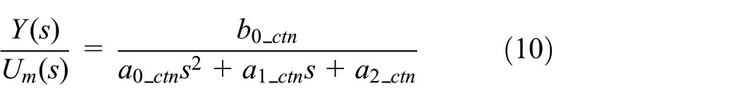
with


Leakage
Depressurizing stage

In predictive controller design, an accurate structure and the parameters of the model are required. In subsystem modeling, many parameters are difficult to measure. It is impossible to accurately describe the model with subjectively estimated parameter values. Therefore, because the model structures of the system are derived, system identification is aimed at estimating the parameters. There are two types of algorithms: in simulations, the reference models are the result of offline identification, which used the recursive least square (RLS) algorithm; in tests, we use the forgetting factor recursive least square (FFRLS) algorithm to perform online identification. For system identification and GPC controller design, the above continuous models must be discretized. The zero-order-hold (ZOH) algorithm is used to transform the continuous models into discrete ARX models

with

In this application, during the pressurizing stage,

where
The estimated parameter vector

The offline identification is a kind of preliminary work: several short-time tests were done; the data of input and pressure were collected, saved, and identified. Because the lengths of data were short, we can set

In actual applications, certain parameters, including bulk modulus, dynamic viscosity, fluid density, and delay, vary slowly in time because they are affected by factors such as environmental temperature, air content of brake fluid, and brake pad wear. GPC controllers are always accompanied by online identifications. Although there are no laws available to predict the parameter variation, the amplitudes of the parameter variation are small. We set λf = 0.999, and
For pressure tracking control, we use 0.01 s control interval in pressurizing GPC controller and 0.02 s in depressurizing controller. It can be sure that the delay time is larger than 0.02 s, if take a larger frequency, the delay compensation length (prediction vector length) would be longer, and the computation would be much more expensive. A set of typical identified models are as follows. For the pressure increasing stage, at a sample time of 0.01 s, we have

with

For the pressure decreasing stage, based on the later discussed equation (39), at sample time of 0.02 s, we have

Figure 8 illustrates a group of response curves of the experimental data and the identified models under the same inputs. The fitting results of the identified models to the unfiltered experimental data were on average 94.8%. We considered the proposed modeling and identification methods to be effective. The identified models accurately represented the actual system and were used as a reference models in later simulations.
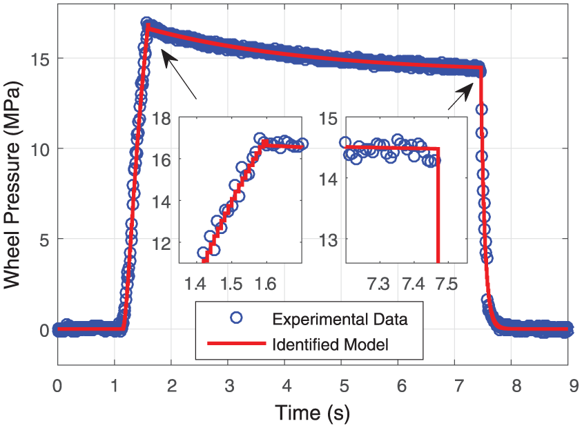
Result of EHB system identification.
Pedal movement
Theoretically, because the pedal and wheel cylinders are decoupled by the PFS, the pressure–displacement (P-D) curve can be customized as needed, and the pedal force–displacement (F-D) relation is the objective of the PFS design process. For comparison to conventional brake systems, we used sets of force–pressure–displacement (F-P-D) experimental data of one vacuum-booster brake (VBB) system as the reference. Although the F-P-D curve during the pedal depressing process differs from that of the pedal releasing process, 15 we use the lookup curve of the depressing stage in PFS design and reference pressure calculation.
PFS
As shown in Figure 9, a passive PFS uses a combination of springs to provide a similar pedal feel to that of VBB systems. The forces acting on the PFS’s piston satisfy the following equation

with

where
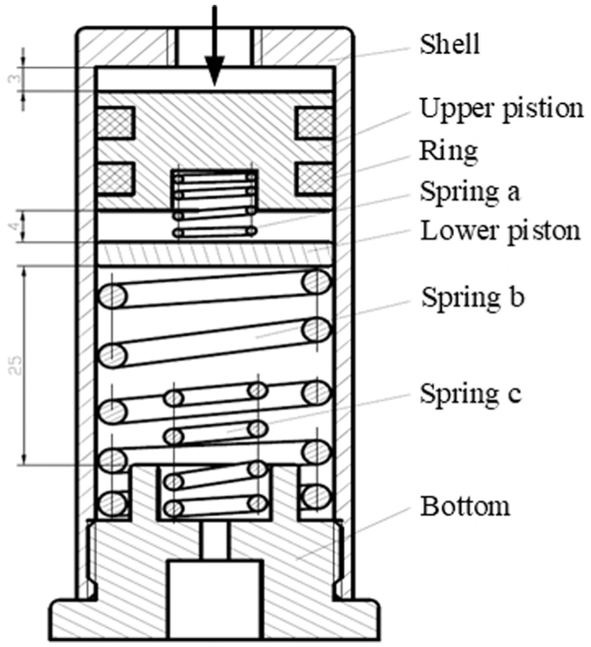
Sectional view of the PFS.
Figure 10 shows two groups of pedal feel test data of the VBB and the PFS and a designed curve of the PFS. The F-D data for the depressing pedal process of the VBB were used to calculate the stiffness of the springs. As shown by the red curve, the F-D curve could be divided into four pieces; except for the preload force of approximately 50 N, the remaining pieces were used to solve for
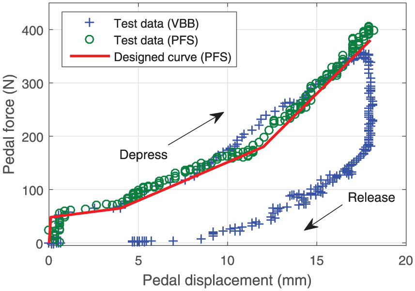
F-D curve of one VBB and the designed PFS.
Reference pressure
For normal brake situations, the reference pressure is calculated from the pedal angle. The relationship between the main cylinder piston displacement

Figure 11 shows the test data of two typical pedal depressing maneuvers in the VBB system. Taking a 2-mm idle travel into consideration, we have the fitted expression

Here,
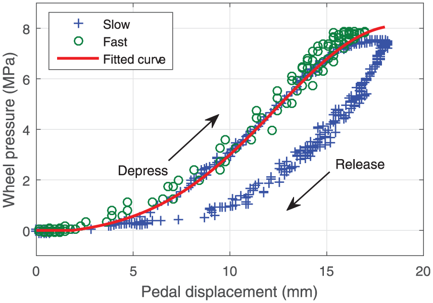
P-D curve in one VBB and the EHB.
Differentiator
Based on Figure 11, due to the restriction of the vacuum structure, the P-D curves of slow and fast pedal depression are almost identical. A conventional VBB system is unable to realize the BA function. When equipped with an active pressure source, for example, the ABS module, common solutions use the combination of the pedal speed and the pedal force as a BA triggering condition for redundancy consideration. 16 However, in a BBW system with a PFS, the relationship between the pedal force and the pedal displacement can be approximately described by a fixed curve. Removing the pedal force sensor has a huge benefit in lowering the cost and minimizing hardware design difficulties. This possibility inspired us to study the method of realizing the BA function using only one angle sensor.
In fact, the research object is the calculation of the differential value of


where
The LD is suitable for a brake system because the internal friction damping limits the maximum pedal speed;
19
thus,
To estimate

Fast pedal (a) depressing and (b) releasing.

Filter performances of the KF and LD methods.
Figure 14 shows the differential values of the raw signal and the KF and LD. In Figure 14(a), the noise of the raw signal is amplified by dividing the sample time; as a result, it is unable to distinguish pedal speed by observing such output data. In Figure 14(b), the differential value of the KF-filtered signals is still too noisy to accurately identify the pedal speed. For Figure 14(c), the output curve shows a clear distinction of movements. Although the LD’s outputs are not absolutely equal to the real speed, we can still use an appropriate threshold value to distinguish fast and slow pedal movements.

Differential outputs of the three methods: (a) differential outputs of raw signals, (b) differential outputs of KF-filtered signals, and (c) differential outputs of LD.
Test verification of the BA function
Here, we use the LD’s output to identify fast or slow depression of the pedal. In the fast depressing mode, the motor will be driven by the maximum power to achieve a greater boost speed, which is expressed as follows

The pedal depression process in Figure 12(a) was adopted to verify BA control. Figure 15 shows the pedal speed during this process. In fact, for the 100 Hz raw signal, noise produces 100 times more disturbance on its differential value. For this sensor, the noise frequency is random and uncertain, and the amplitudes of the noise are approximately equal to the sensor’s minimum accuracy or its integral multiples (in this sensor, the minimum accuracy is approximately 0.1 mm, but it may vary under different working environments). From Figure 15, we can find that the amplitude of the noise differential is approximately 20 mm/s. However, as shown by the red curve, the negative oscillation of the differential value is significantly suppressed. When the pedal began to move at 0.7 s, the differentiator output exceeds +10 at 0.8 s, that is, there is an acceptable 0.1 s delay.

Differential output during a fast pedal depressing maneuver.
Figure 16 shows a group of measured pressures in the BA tests. By observing the blue curve, because the pedal rod has a rigid connection with the hydraulic loop, the pressure response of VBB has a smaller delay than that of EHB. However, regardless of how fast the pedal is depressed, the relationship between pressure and displacement remains unchanged. For EHB with BA control, the pressure is less than that of the VBB in the initial 0.2 s. For BA, by triggering for a period of 0.8–1.3 s, the EHB outputs the maximum power. After a transport delay, the BA’s pressure exceeds that of no BA at 0.84 s and that of the vacuum booster at 0.88 s and then reaches a maximum pressure soon thereafter. This control method can be considered both feasible and effective.

Experimental verification of BA control.
Controller design
Normally, many applications use an inner current loop to indirectly control the motor torque because the current has an approximately proportional relationship to the load torque. However, there are a few reasons why we do not use current-loop control: (1) the brake pressure can be regarded as the load on the motor pump, thus eliminating the need to estimate torque through the current when using pressure sensors; (2) when the motor’s eccentric shaft is rotating, the force acting on the piston vibrates cyclically, and, accordingly, the current oscillates, making it difficult to use such current to control torque precisely; and (3) because of the effect of operating temperatures on the motor starting current and pump internal friction variation, it is difficult to identify an accurate fixed relation between the current and the load torque via calibration tests. In this article, the control object in the pressurizing stage is the motor speed, which controls the pressurizing rates and time. The existing PWM speed control technique is mature and suitable for this application.
Safety is the priority of brake systems. A faster response corresponds to a shorter brake distance. A consistent relationship between a vehicle’s brake force and a driver’s brake pedal input leads to a comfortable and confident brake feel. The large pressure overshoots may lead to an unnecessary triggering of the ABS and extension of the actuator working time. Previously, several PID parameter combinations were attempted. Clearly, stable PID controllers exist; however, the response time of such controllers is longer. When the actual pressure is close to the reference pressure, the stable PID controller would then take more time to reach the reference. If the derivative effect of the PID is weakened, overshoots would emerge again.
To address this dilemma, predictive control was found to be the optimum method. Figure 17 shows the schematic diagram of the control loop (in this section, the BA function is not used). The GPC controllers contain two sub-controllers: a motor and reducing valve; each controls the pressure increase or decrease process. The EHB block can switch between the simulation model and the test bench.

Control flow scheme of the simulation and the test.
GPC algorithm
Taking the pressurizing stage as an example, although the mechanical model of the motor pump has dynamic nonlinearity, the pressure increasing model could still be expressed as a linear model when

By transforming equation (25) to an incremental form, we have

with

where
The prediction model at the sample time

where

with

The prediction error at

Its variance can be expressed as follows

The optimal prediction error

We define a quadratic cost function as follows

with

where
Based on equation (27),

with


Substituting equation (33) into equation (32), for

Note that the driving voltages of the motor and valves are limited. When constraints exist,
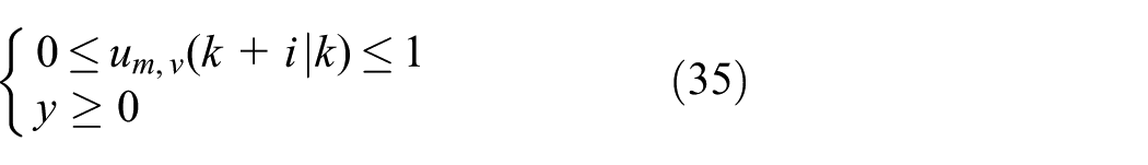
Transforming the constraint into incremental form, we have

with


Substituting equation (27) into equation (32), the general quadratic programming form is obtained

with
To solve the quadratic cost function defined by equation (34) under the constraint equation (36), the Quadratic Programming algorithm using Active Set iterations was utilized. The specific algorithms were discussed in the previous studies.20,21
When compared to single-step optimization controllers, the multi-step optimization of GPC has better robustness. When the
Pressurizing controller
The issue of choosing the controller parameters is analyzed via simulation. Theoretically, the step response will have a maximum overshoot at the maximum slope point of the step response curve. We choose 8 MPa as a reference pressure to simulate the control effects at different

Pressurizing response at different Np.

Controller outputs at different Np.
The response speed and overshoot are usually incompatible, especially in this non-minimum phase system. Nevertheless, by taking advantage of the GPC properties and the dynamic nonlinear characteristic of the motor pump, it is feasible to find a balance between rapidity and accuracy. The motor pump pushes the fluid unidirectionally, and there is almost no inertia effect, that is, when the prediction output
The control effects of different

Pressurizing response at different N u .
Depressurizing controller
The PWM carrier frequency of the valve and its controller frequency are both 50 Hz. We use 1000 Hz as the RCP test frequency to ensure at least 5% of the duty ratio is adjustable. For the nonlinear model of the depressurizing stage (equation (12)), the pressure output
We have a

Figure 21 shows the simulation results of different

Depressurizing response at different Np.
Additional error dead-zone control
Under normal braking conditions, the EHB system model contains a double input

where
The introduction of control dead-zone could not only reduce the start–stop frequency of the actuators but also restrain the overshoot caused by the delay. As shown in Figure 22, the GPC and PID controllers without the dead-zone strived to lower the error to 0 and caused the pressure fluctuate near the reference. Alternatively, by observing the pressure curve of the PID controller with the dead-zone, some overshoots are greater than the dead-zone range; thus, there are still a few adjusting cycles. The GPC controller with the dead-zone allows small overshoots to increase and has an earlier stopping time when decreasing. Figure 23 shows the outputs
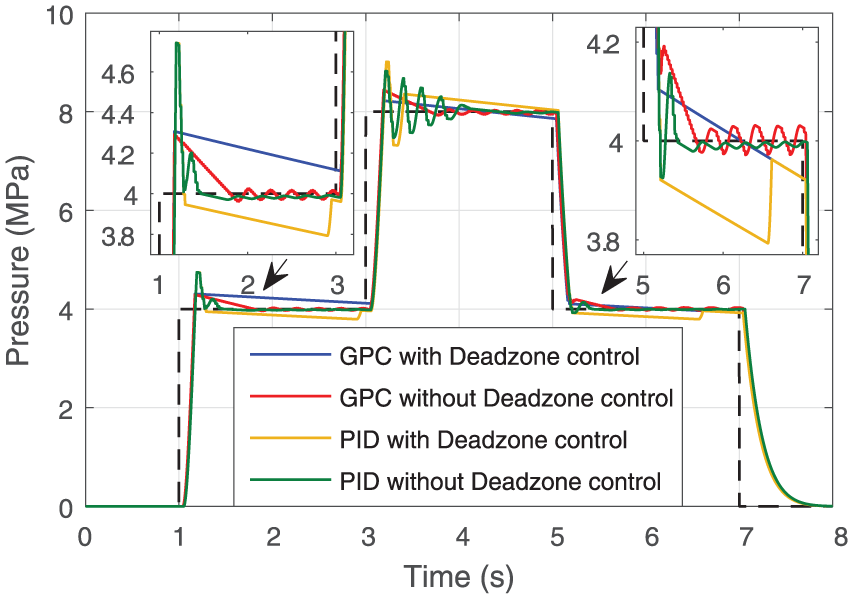
Tracking performance of four methods.

Comparison of the outputs of four controllers:(a) GPC with dead-zone control, (b) GPC without dead-zone control, (c) PID with dead-zone control, and (d) PID without dead-zone control.
Test verification of the pressure tracking
Static closed-loop tests (wheels remain static) were performed to evaluate the tracking performance of the wheel pressure. The results of two typical brake maneuvers are shown in Figures 26 and 27. For comparison, two earlier test results using well-tuned PID controllers are plotted in Figures 24 and 25. Figure 24 shows the tracking result when the driver depresses the pedal slowly. Several positive and negative overshoots can be identified. Figure 25 shows a tracking result of slow pedal release. Similarly, in the periods of 4 to 6 s and 9 to 10 s, repeating pressure vibrations are found. During these periods, the motor and reducing valve were driven alternately to adjust the pressure and achieve the reference pressure. From these two figures, the pressure tracking of the PID controller is more likely to exhibit unsteady pressure vibration.

Experimental tracking result of slow pedal depression (PID).

Experimental tracking result of slow pedal release (PID).
In Figures 26 and 27, the tracking performances of the proposed controller are evaluated with slow pedal depression and release. There are nearly no overshoots. In Figure 26, at the increasing stage of the prior 4 s, compared to the reference pressure, the measured pressure does not fluctuate frequently. In the period between 4 and 7 s, the controller outputs of the motor and the reducing valve are

Experimental tracking result of slow pedal depression (GPC).

Experimental tracking result of slow pedal release (GPC).
From the above tests, we can conclude the following: (1) the proposed GPC controllers have fine tracking performance; (2) the design of the error dead-zone control method promotes the anti-jamming property effectively, and when controllers of the motor and reducing valve ignore the small error
Conclusion
This article presented a novel EHB system. The characteristics and pressure control of the prototype were illustrated through simulation and RCP tests. The main results and conclusions are as follows:
Considering the brake pedal characteristics, when the pedal maximum speed can be estimated, the LD is suitable for the BA function of the EHB. This approach may provide a new method for lowering the cost and reducing the algorithm complexity. Although accumulator-type EHBs have better pressure boost ability, the proposed EHB can still have a preferable performance in practical application with the help of BA.
The proposed identification method proved to be effective; therefore, GPC controllers were introduced to optimize the pressure tracking performance. When compared with a PID controller, simulations and test results showed that a GPC controller has apparent advantages. Most of the time, GPC controllers output the maximum driven voltage in the pressure tracking process and stop in a timely manner when reaching the reference pressure. The control effect could achieve a balance between rapidity and accuracy. Moreover, the benefits of service life and energy savings are achieved.
Footnotes
Acknowledgements
The authors would like to thank the reviewers and the Associate Editor for their helpful and detailed comments, which have helped to improve the presentation of this article.
Handling Editor: Fakher Chaari
Declaration of conflicting interests
The author(s) declared no potential conflicts of interest with respect to the research, authorship, and/or publication of this article.
Funding
The author(s) disclosed receipt of the following financial support for the research, authorship, and/or publication of this article: This work was financially supported in part by the National Natural Science Foundation of the People’s Republic of China (grant number: 51505354).