Sage Journals: Discover world-class research

Abstract

Reversible axial-flow pump is widely adopted in the coastal regions or along the river. Due to severe vibration, which results in impeller cracks in unstable region, the fluid–structure interaction solving strategy of impeller was applied for reversible axial-flow pump. In unstable region, the two-way coupling method was employed to obtain the pump performance curve and the quantity analysis of deformation and stress on impeller. The results show that the measured efficiency and head are in good agreement with the simulation values. Under positive rotation, the maximum equivalent stress and total deformation are found to be below 0.75Q _des. Under negative rotation, the maximum total deformation is observed to be below 0.65Q _des and the maximum equivalent stress increases with increase in flow rate. Whether under positive or negative rotation, along the direction from impeller inlet to outlet and in the direction from impeller hub to rim, the total deformation goes up and the equivalent stress first increases and then declines. The results indicate that the equivalent stress reduces with decrease in fillet radii. The analysis results of deformation and stress can be utilized to guide the structure design of reversible axial-flow pumps and attain more stable pump performance.

Keywords

Reversible axial-flow pump unstable region fluid–structure interaction total deformation equivalent stress

Introduction

Reversible axial-flow pump, as an important part of water conservancy projects, can change the flow direction by changing the rotation direction of impeller. Therefore, it can meet both the needs of drainage and water transfer, and it is widely used in the coastal regions or along the river. However, under small flow rate condition (below 70% design flow rate¹), there is unstable operation region where severe vibration and noise will be produced and the pump head will drop rapidly with increasing flow rate. In unstable operation region, there is strong interaction between impeller structure and turbulent flow, which will cause complex deformation of impeller structure and even cracks. Therefore, in axial-flow pumps, many scholars are devoted to the study of the flow pattern in unstable region^2–4 to find methods to eliminate the phenomenon of instability flow.⁵ To ensure safe operation of axial-flow pump for every flow rate, the analysis of stress and deformation on impeller in unstable operation region need to be solved by consideration of fluid–structure interaction (FSI).⁶

In recent times, with the extensive application of computational fluid dynamics (CFD),^7–10 there are some researches on FSI in fluid machineries such as turbine,^11–13 compressor and pump. Langthjem and Olhoff¹⁴ simulated the flow-induced noise in a two-dimensional (2D) centrifugal pump and analyzed the influence of the FSI between inner flow and impeller on noise generation. Landvogt et al.¹⁵ calculated the pressure distribution in a new axial hydraulic pump by considering FSI to find an optimal layout of compensation chamber and pump. Benra et al.^16–18 used different coupling methods of FSI to study the oscillations of single-blade impeller in sewage water pump and the numerical results for different methods were compared with experimental data to verify the feasibility. Kobayashi et al.¹⁹ investigated a mixed-flow pump with unshrouded impeller by one-way coupled FSI and the distribution of stress on impeller was obtained. Yuan et al.²⁰ used two-way coupling method to study the effect of FSI on radial forces, pressure distribution, equivalent stress and rotor deflection in a centrifugal pump. Schneider et al.²¹ quantitatively analyzed the distribution of stress and deformation in impeller of multistage pump considering FSI. Pei et al.^22,23 calculated dynamic stresses on a single-blade centrifugal pump impeller considering FSI and the calculation accuracy was verified by impeller oscillation measurement. It is known that reversible impeller plays an important role in reversible axial-flow pump. In order to ensure the pump efficiency under positive and negative rotation, the inlet and outlet angles of reversible impeller are set to be the same. Due to the special shape of the impeller, the distribution of stress and deformation on reversible impeller may have much variation. In addition, both the distribution of stress and deformation on impeller under positive and negative rotation need to be taken into account. However, there is little research on analysis of stress and deformation for reversible axial-flow pump considering FSI, especially in the unstable region.

In this study, the interaction between turbulent flow and impeller structure is simulated for a reversible axial-flow pump by using a two-way coupling method. The equivalent stress and total deformation distribution on the reversible impeller were calculated under both positive and negative impeller rotation conditions.

Mathematical model and FSI setup

Pump and system parameters

The three-dimensional (3D) model of reversible axial-flow pump, which consists of inlet section, reversible impeller, straight guide vane and outlet section, is shown in Figure 1. The impeller hub diameter is 98 mm, and the outer diameter and tip clearance of impeller is 300 and 0.5 mm, respectively. The number of both impeller blade and guide vane blade is 3. The pump design parameters and the structure material parameters are as listed in Table 1.

Figure 1.

3D model of reversible axial-flow pump.

Table 1.

Parameters of reversible axial-flow pump.

Design parameters	Design flow rate, Q _des (l/s)	Rotation speed, n (r/min)	Design head, H (m)
	28	1104	1.57
Material parameters	Density, ρ (kg/m³)	Poisson ratio, μ_p	Elastic modulus, E (GPa)
	7850	0.3	200

Approach of coupled solution

There are three different approaches to FSI simulation system, based on the literature²¹ (monolithic approach, loose coupling of partitioned approach and strong coupling of partitioned approach). In this study, the strong coupling of partitioned approach was applied as shown in Figure 2. The computational domain includes both fluid and solid domains. First, the fluid domain was computed using the finite volume method and the calculated force load was transferred through fluid–solid interface to the solid part. Second, the solid part was calculated by finite-element method (FEM) for which the force load was set as boundary condition. Finally, the FSI calculation convergence was checked considering all the load components transferred between two parts individually. If the calculation convergence reached the convergence target, the FSI iteration would begin the next time step. Otherwise, the FSI iteration would continue for the current time step.

Figure 2.

Flow chart of FSI simulation.

Calculation grids and boundary conditions

The structure grids of inlet section, impeller, guide vane, and outlet section are generated by ICEM-CFD 14.5 as shown in Figure 3(a). As shown in the figure, when the total number of grid nodes for all fluid domains is less than 6.34 × 10⁶, the head increases rapidly with increase in grid number. However, when the grid number is more than 6.34 × 10⁶, the head remains stable while the number grid increases. In order to save computing resource, the grid number was selected as 6.34 × 10⁶. Unsteady flow considering FSI was simulated using the Reynolds-averaged Navier–Stokes (RANS) equation with shear stress transport (SST) k–ω turbulence model. The maximum number of Y plus was 94 for the entire computational domain. The boundary condition for inlet and outlet was set as mass flow rate and static pressure, respectively. The interface boundary conditions between inlet section and impeller, and impeller and guide vane were set as “transient rotor-stator” to consider the transient interaction in the flow between rotor and stator. The interface boundary condition between guide vane and outlet section was set as “none.” The wall function was set as the smooth wall with no-slip condition. Under design rotating speed, the time step was set as 1.51 × 10⁻⁴ s and the rotating angle within each time step was set as Δϕ = 1. In order to ensure the accuracy and reliability of numerical simulation, the maximum residual was set as 10⁻⁴ and the total time for unsteady simulation and coupling numerical calculation was 0.435 and 0.326 s, respectively.

Figure 3.

Mesh of the CFD model: (a) grid of fluid domain and (b) analysis of grid independence.

The impeller of solid domain is shown in Figure 4, and all surfaces of blades were set as fluid–structure interface and the fixed support was used on the surface of impeller hub. The grid number of solid domain is 52,746. The coupling surface was used to transfer the data between fluid and solid domains. Because of the different mesh node numbers for CFD and FEM model, the deformation transfer and force transfer were set as preserving interpolation and conservative interpolation, respectively. The convergence target for the load transfer is 0.01 and the under-relaxation factor was set as 0.75 for the external load transfer parameters. In interpolation mapping, the fluid–structure interface for fluid domain and solid domain had good agreement and the non-matching area fractions are less than 0.5%, which can be used to ensure the accuracy of data transmission.

Figure 4.

Constraints of reversible impeller.

Experimental validations

Figure 5 shows the closed-loop test bench with bidirectional shaft tubular pump model, which consists of an electric valve, pressure tank, a butterfly valve, an electromagnetic flowmeter, a torque meter and a pressure transmitter. The measurement uncertainty of intelligent electromagnetic flowmeter measurement, ZJYW1/ZJ 200-Nm torque meter and WT2000DP5S intelligent pressure sensor were ± 0.2%, ± 0.14% and ± 0.1%, respectively. The measurement uncertainty of the test bench system was ±0.26%, which complied with national standards. Figure 6 shows the performance curve of pump under positive and negative rotation, and the saddle curve of head was obtained between 0.55 and 0.75Q _des (under both positive and negative rotation). The simulated efficiency and head was calculated by two-way coupling method. Good agreement between simulated and measured value was obtained. So the simulated results are reliable and reasonable.

Figure 5.

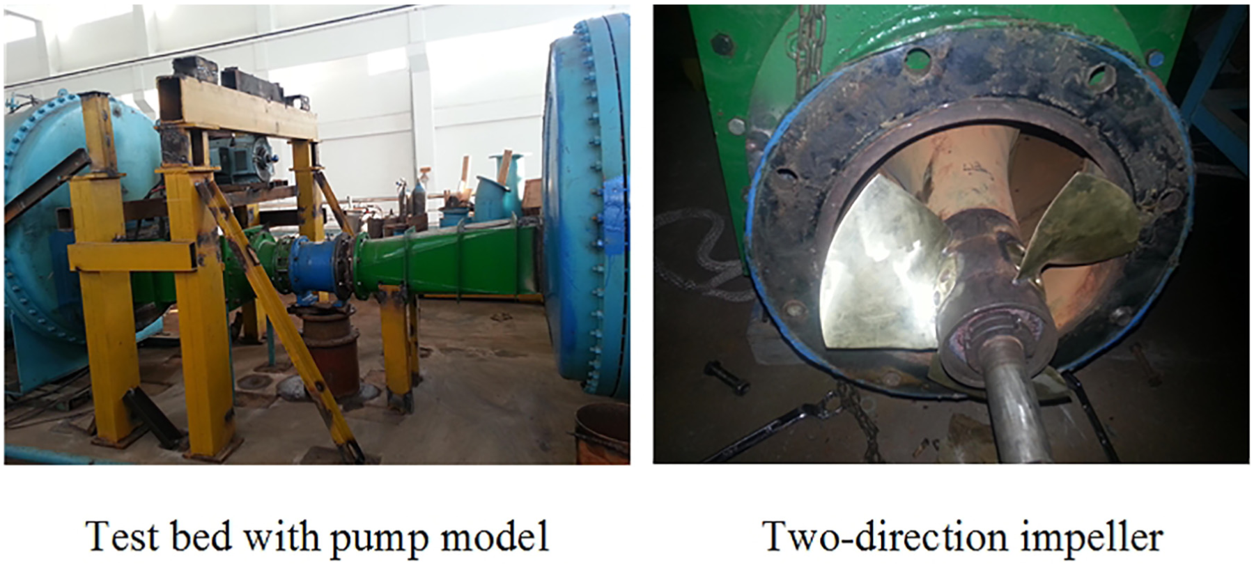
Photograph of test bed with reversible axial-flow pump model.

Figure 6.

Performance curve of pump under (a) positive rotation and (b) negative rotation.

Results and discussion

Figure 7(a) shows the maximum total deformation and equivalent stress for different flow rates under positive rotation condition. The total deformation and equivalent stress first rise and then decline with increasing flow rate, and the highest points of both are found to be at 0.75Q _des. Figure 7(b) shows the maximum total deformation and equivalent stress for different flow rates under negative rotation condition. The total deformation appears fluctuating with increasing flow rate and the highest point can be obtained at 0.65Q _des. However, the equivalent stress rises with increasing flow rate. (The total deformation and equivalent stress is defined as the maximum value at every time step.)

Figure 7.

Maximum total deformation and equivalent stress for different flow rates under: (a) positive rotation and (b) negative rotation.

The distribution of total deformation on impeller surface under positive rotation and negative rotation are shown in Figure 8(a) and (b), respectively, which is viewed from the impeller inlet. The total deformation increases from impeller hub to impeller rim, and the maximum can be found at the junction of impeller rim and impeller blade inlet. The distribution of equivalent stress on impeller surface under positive rotation and negative rotation are shown in Figure 9(a) and (b), respectively, which is viewed from the impeller inlet. The high stress region is close to impeller inlet and impeller hub and the area of high stress region at 0.75Q _des is the largest. Furthermore, the maximum can be obtained near the impeller inlet. Due to the instability of internal flow, the distribution of total deformation and equivalent stress on each impeller blade is not the same.

Figure 8.

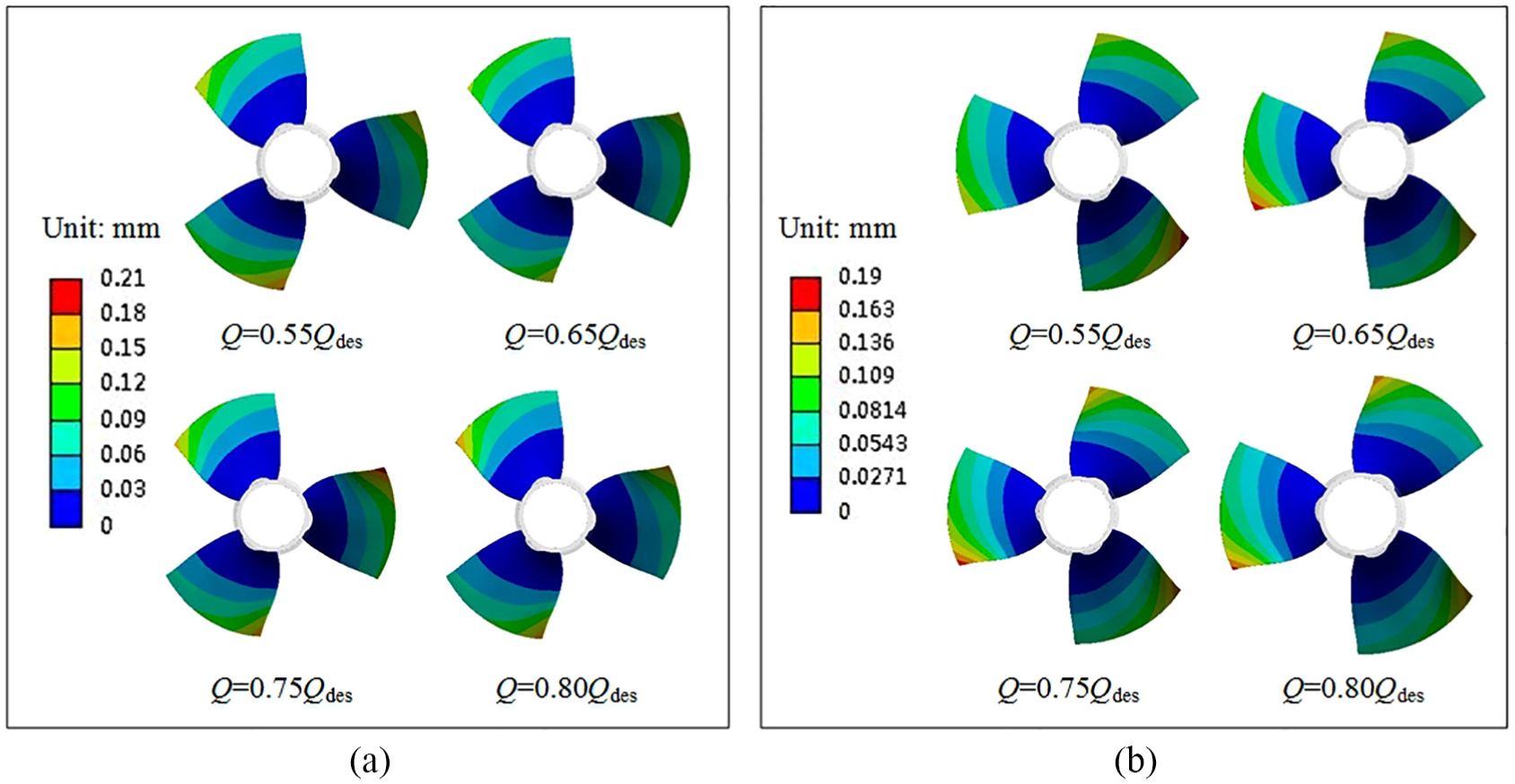
Distribution of the total deformation on impeller surface under (a) positive rotation and (b) negative rotation.

Figure 9.

Distribution of the equivalent stress on impeller surface under (a) positive rotation and (b) negative rotation.

The paths are defined to study the trend of total deformation and equivalent stress with fillet radii in unsteady region. As shown in Figure 10, the ps, ss Le, and Tr are short for pressure side, suction side, leading edge, and trailing edge, respectively. The Le-ps, Le-ss, Te-ps, and Te-ss represent the direction from hub to rim. In addition, the Hub-ps, Hub-ss, Rim-ps, and Rim-ss represent the direction from leading edge to trailing edge. According to the critical regions of large total deformation and high equivalent stress, the total deformation distribution on fillet radii paths of Rim-ps, Rim-ss, Le-ps, and Le-ss, and the equivalent stress distribution on fillet radii paths of Hub-ps, Hub-ss, Le-ps, and Le-ss need to be investigated.

Figure 10.

Investigated paths in the fillet radii (under positive rotation).

In the following analysis, the total deformation and equivalent stress are defined as the maximum value of each point along the paths at every time step. Figure 11 shows the distribution of total deformation in fillet radii paths under positive rotation. In the paths of Rim-ps and Rim-ss, the total deformation reduces from impeller inlet to impeller outlet, and the values are the largest and the smallest at 0.75 and 0.80Q _des, respectively. In the paths of Le-Ps and Le-Ss, the total deformation first remains stable and then increases from impeller hub to impeller rim. The values of total deformation at 0.75Q _des are the largest and that at other flow rates are close. Figure 12 shows the distribution of equivalent stress in fillet radii paths under positive rotation. The equivalent stress appears to fluctuate and the maximum value can be found to range from path length = 0.4–0.6. In the paths of Hub-ps and Hub-ss, the values of equivalent stress at 0.80Q _des are the smallest and that at other flow rates are close. In the paths of Le-ps and Le-ss, the values at 0.75 and 0.55Q _des are the largest and the smallest, respectively.

Figure 11.

Distribution of total deformation in fillet radii paths for different flow rates under positive rotation.

Figure 12.

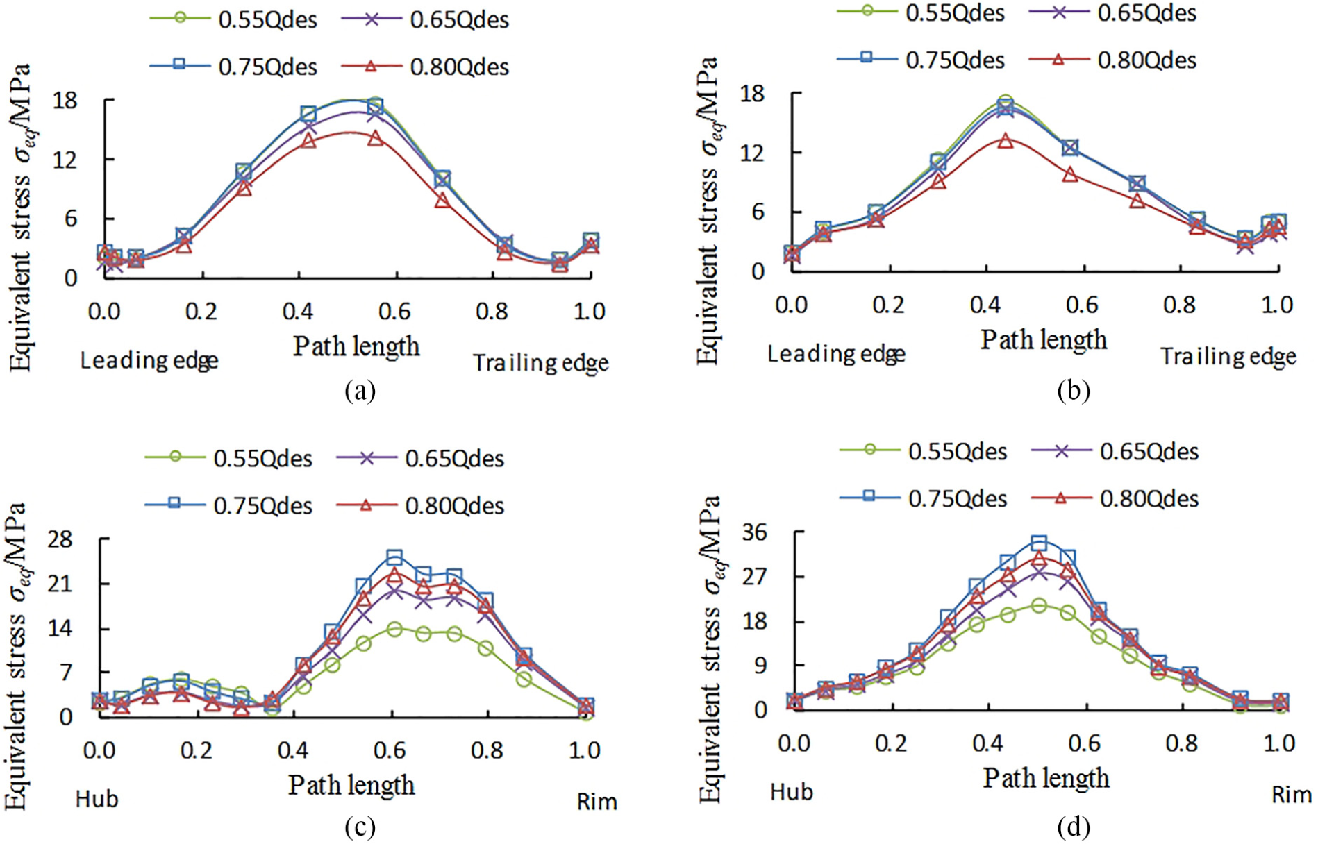
Distribution of equivalent stress in fillet radii paths for different flow rates under positive rotation.

Figure 13 shows the distribution of total deformation in fillet radii paths under negative rotation. In the paths of Rim-ps and Rim-ss, the total deformation increases form leading edge to trailing edge, and the values below 0.65Q _des are the largest. In paths of Te-ps and Te-ss, the total deformation first remains stable and then increases from hub to impeller rim and the values at 0.55Q _des are the smallest. Figure 14 shows the distribution of equivalent stress in fillet radii paths under negative rotation. The equivalent stress shows fluctuation and the maximum can be obtained in range from path length = 0.4 to 0.6. In the paths of Hub-ps and Hub-ss, the values are the largest and the smallest at 0.6 and 0.80Q _des, respectively. In the paths of Te-ps and Te-ss, the values at 0.55Q _des are the smallest.

Figure 13.

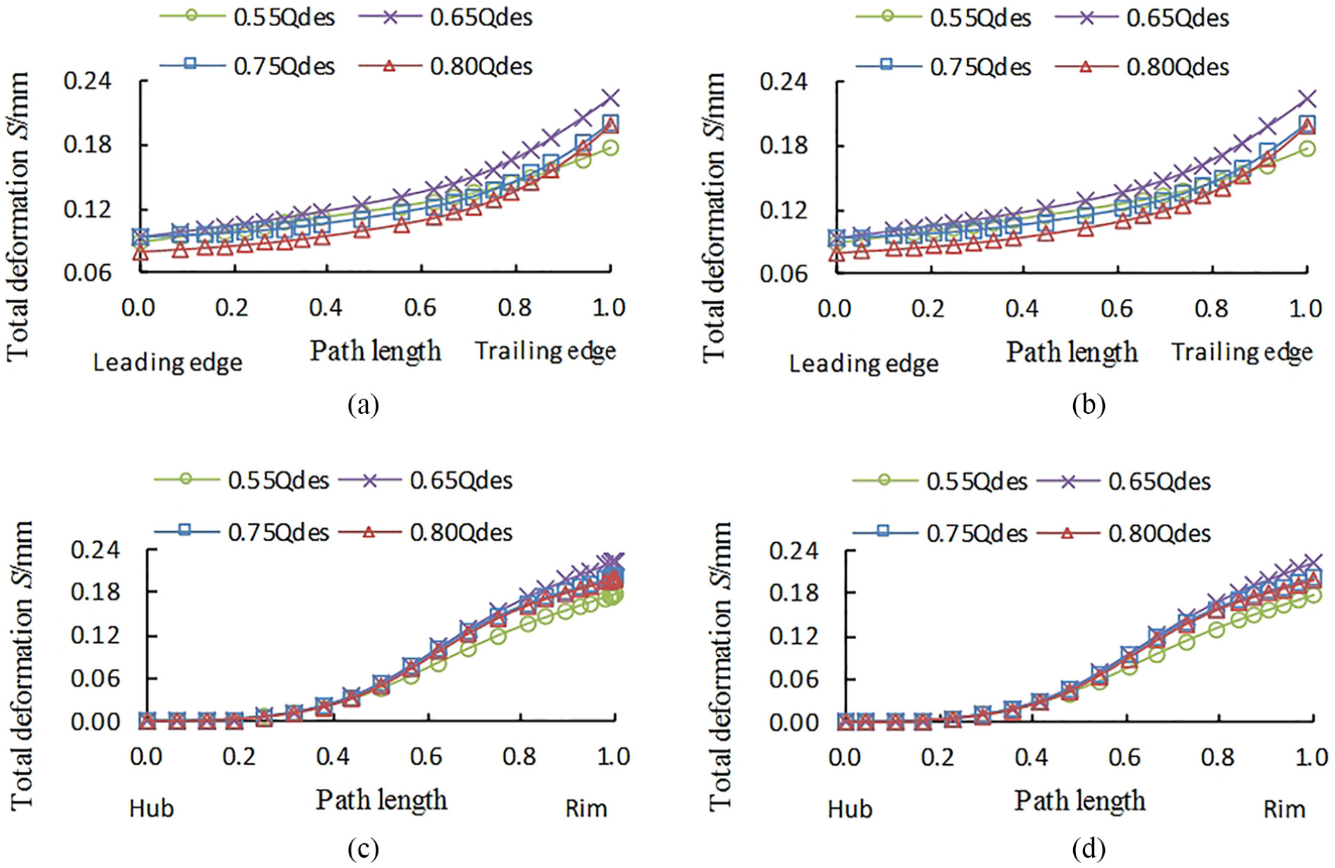
Distribution of total deformation in fillet radii paths for different flow rates under negative rotation.

Figure 14.

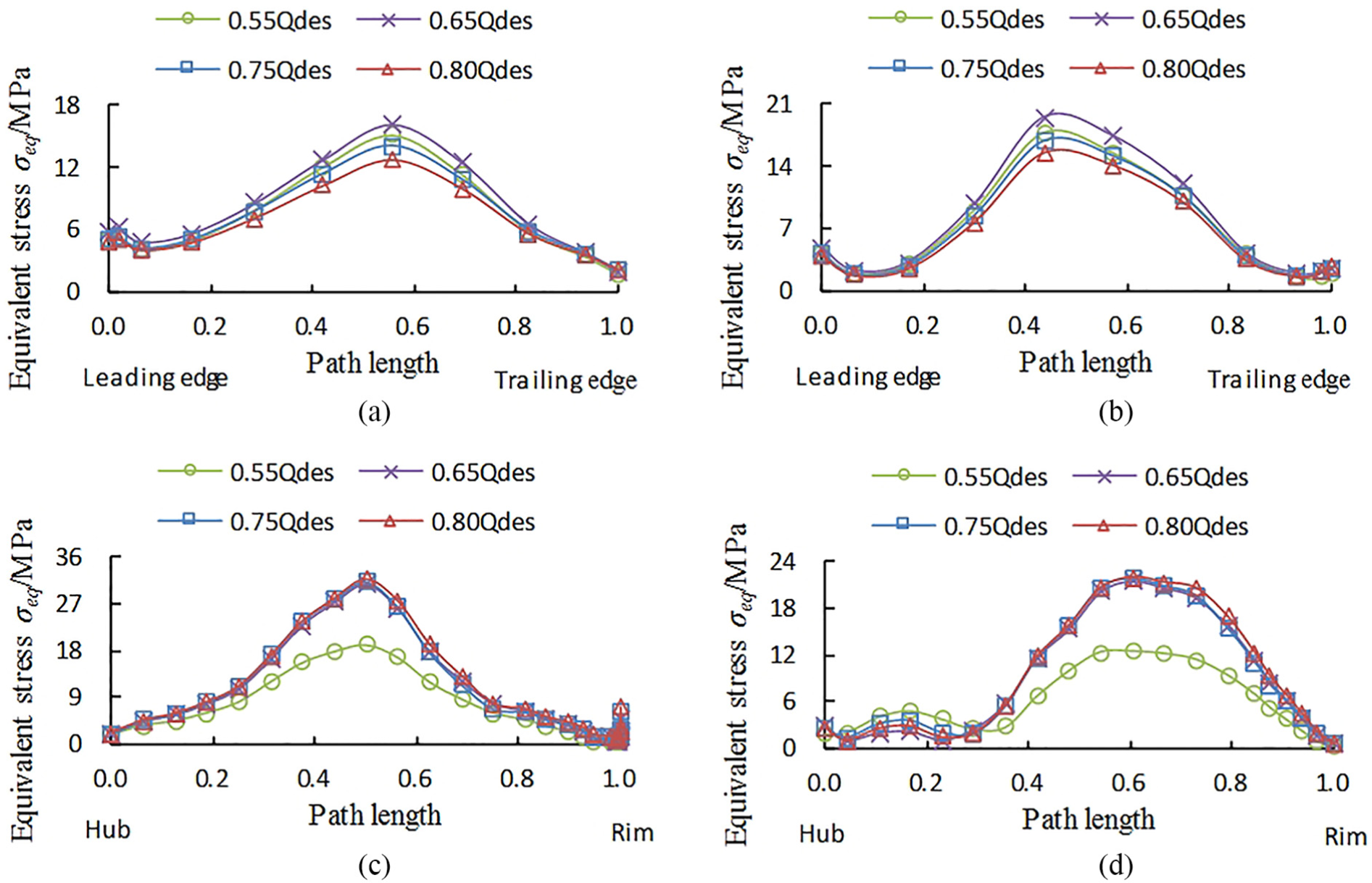
Distribution of equivalent stress in fillet radii paths for different flow rates under negative rotation.

The analysis of total deformation and equivalent stress on fillet radii paths indicated that the equivalent stress reduced with decrease in fillet radii, but the total deformation was mainly influenced by flow field, under both positive and negative rotation.

Conclusion

In order to obtain the distribution of total deformation and equivalent stress on impeller surface in unsteady region, the coupled solution of the flow field and structural response of the impeller was established. The conclusions drawn are as follows:

The unsteady region is found in the range of flow rate from 0.55 to 0.75Q _des. The maximum total deformation and equivalent stress on impeller were significantly affected by the flow rate. Under positive rotation, the equivalent stress and total deformation of impeller blade at 0.75Q _des is the largest, while under negative rotation, the largest total deformation appeared below 0.65Q _des and the equivalent stress increased with increase in flow rate.

The total deformation on the surface of impeller blade increases from impeller hub to rim and the maximum can be found near the junction of impeller inlet and rim. Near the region of the impeller hub and inlet, on the surface of impeller blade, there is strong equivalent stress.

The total deformation in the paths of impeller rim decreases from impeller inlet to outlet, and that in the paths of leading edge increases from impeller hub to rim, which means the total deformation was mainly affected by the flow field. The maximum equivalent stress in the paths of impeller hub and impeller inlet can be obtained in the middle of these paths, which indicates that the equivalent stress reduces with decrease in fillet radii.

The knowledge of distribution of deformation and stress and the maximum area can provide guide information about structure design of impeller shape to ensure pump reliability.

Footnotes

Handling Editor: Farzad Ebrahimi

Declaration of conflicting interests

The author(s) declared no potential conflicts of interest with respect to the research, authorship, and/or publication of this article.

Funding

The author(s) disclosed receipt of the following financial support for the research, authorship, and/or publication of this article: The authors are deeply grateful for the financial support of this study by the Jiangsu Province of Science and Technology (BY2016072-05) and the National Science and Technology supporting plan (2015BAD20B01).

References

Perez Flores

Kosyna

Wulff

. Suppression of performance curve instability of an axial-flow pump by using a double-inlet-nozzle. Int J Rotat Mach 2008; 2008: 536850.

Goltz

Kosyna

Stark

et al . Stall inception phenomena in a single-stage axial-flow pump. Proc IMechE, Part A: J Power and Energy 2003; 217: 471–479.

Chen

Feng

Zhou

et al . Effects of inlet guide vane on characteristics of backflow vortex in hump region of axial flow pump. Trans Chin Soc Agric Mach 2016; 47: 8–14 (in Chinese).

Zheng

Chen

Zhang

et al . Analysis on unsteady stall flow characteristics in axial-flow pump. Trans Chin Soc Agric Mach 2017; 48(7): 127–135 (in Chinese).

Goltz

Kosyna

Delgado

. Eliminating the head instability of an axial-flow pump using axial grooves. Proc IMechE, Part A: J Power and Energy 2013; 227: 206–215.

Piperno

Farhat

Larrouturou

. Partitioned procedures for the transient solution of coupled aroelastic problems part I: model problem, theory and two-dimensional application. Comput Method Appl M 1995; 124: 79–112.

Sun

Zuo

Liu

et al . Distribution of pressure fluctuations in a prototype pump turbine at pump mode. Adv Mech Eng 2014; 6: 923–937.

Zou

et al . Numerical investigation of degas performance on impeller of medium-consistency pump. Adv Mech Eng 2015; 7: 1–9.

Jiang

Pang

et al . Numerical simulation and performance analysis of a four-stage centrifugal pump. Adv Mech Eng 2016; 8: 1–8.

10.

Zhang

Guo

Wang

. Large eddy simulation of turbulent flow in a true 3D Francis hydro turbine passage with dynamical fluid–structure interaction. Int J Numer Meth Fl 2007; 54: 517–541.

11.

et al . Experimental and numerical study of transient flow in a centrifugal pump during startup. J Mech Sci Technol 2011; 25: 749–757.

12.

Campbell

Paterson

. Fluid–structure interaction analysis of flexible turbomachinery. J Fluid Struct 2011; 27: 1376–1391.

13.

Zhang

Guo

Wang

. FEM simulation of turbulent flow in a turbine blade passage with dynamical fluid–structure interaction. Int J Numer Meth Fl 2009; 61: 1299–1330.

14.

Langthjem

Olhoff

. A numerical study of flow-induced noise in a two-dimensional centrifugal pump. Part I. Hydrodynamics. J Fluid Struct 2004; 19: 349–368.

15.

Landvogt

Osiecki

Patrosz

et al . Numerical simulation of fluid-structure interaction in the design process for a new axial hydraulic pump. Prog Comput Fluid Dy 2014; 14: 31–37.

16.

Benra

. Application of fluid/structure interaction methods to determine the impeller orbit curves of a centrifugal pump. In: Proceedings of the 5th IASME/WSEAS international conference on fluid mechanics and aerodynamics, Athens, Greece, 25–27 August 2007, pp.169–174.

17.

Benra

. Numerical and experimental investigation on the flow induced oscillations of a single-blade pump impeller. J Fluid Eng: T ASME 2006; 128: 783–793.

18.

Benra

Dohmen

Wan

. Determination of pump impeller deflections: comparison of FSI-simulations to measurements. In: Proceedings of the ASME FEDSM, Miami, FL, 17–20 July 2006. New York: ASME.

19.

Kobayashi

Ono

Harada

et al . Numerical analysis of stress on pump blade by one-way coupled fluid-structure simulation. J Fluid Sci Tech 2010; 5: 219–234.

20.

Yuan

Pei

Yuan

. Numerical investigation on fluid structure interaction considering rotor deformation for a centrifugal pump. Chin J Mech Eng 2011; 24: 1–7.

21.

Schneider

Will

Böhle

. Numerical evaluation of deformation and stress in impellers of multistage pumps by means of fluid structure interaction. In: Proceedings of the ASME 2013 fluids engineering division summer meeting, Incline Village, NV, 7–11 July 2013. New York: ASME.

22.

Pei

Yuan

. Dynamic stress analysis of sewage centrifugal pump impeller based on two-way coupling method. Chin J Mech Eng 2014; 27: 369–375.

23.

Pei

Yuan

. Fluid-structure coupling effects on periodically transient flow of a single-blade sewage centrifugal pump. J Mech Sci Technol 2013; 27: 2015–2023.

Fluid–structure coupling analysis of impeller in unstable region for a reversible axial-flow pump device

Abstract

Keywords

Introduction

Mathematical model and FSI setup

Pump and system parameters

Approach of coupled solution

Calculation grids and boundary conditions

Experimental validations

Results and discussion

Conclusion

Footnotes

Declaration of conflicting interests

Funding

References