Sage Journals: Discover world-class research

Abstract

Axial-flow pump with a two-way passage has been widely employed in irrigation and drainage projects. Because of the shape of the two-way inlet passage, the impeller easily induces vibration due to unstable turbulent flow. This vibration results in structural cracks and even hinders the safe operation of the pump. Deformation and stress distributions in the impeller were calculated using two-way coupled fluid–structure interaction simulations, and a quantitative analysis of blade deformation and stress is carried out to determine the structure critical region. The results show that the values of deformation and stress significantly decrease with an increasing flow rate and a decreasing head, and the maximum total deformation can be found in the impeller rim, while the maximum equivalent stress can be obtained near the impeller hub. The total deformations in the blade rim decrease from blade leading edge to trailing edge, and the equivalent stress in the blade hub initially increases and then declines, and in the end, it rapidly increases from the blade outlet to inlet. These results reveal the deformation and stress in the impeller to ensure reliability and specific theoretical guidance for the structural optimization design of a pump device.

Keywords

Axial-flow pump fluid–structure interaction total deformation equivalent stress flow-induced vibration

Introduction

An axial-flow pump device with a two-way passage consists of an impeller, a guide vane, a two-way inlet passage, and a two-way outlet passage. Because of its advantages of a small floor area and easy maintenance, it is often adopted to meet the demand of a large farmland and the associated drainage. However, a vortex is easily formed in the two-way inlet passage. The bad flow state in the inlet passage will lead to flow separation and, in turn, a vortex in the impeller, which may cause impeller vibration (deformation and stress problems). These problems will lead to degradation of the pump device performance, thus hindering its safe operation. Fluid–structure interaction (FSI) produced this phenomenon. Therefore, determining the stress distribution and deformation in the impeller to ensure the reliability of the pump device requires not only a solution for the internal flow field of the pump but also an analysis of the structural mechanics of the impeller.

In recent years, an increasing number of researchers have begun to apply the theory of fluid–solid coupling to turbomachinery^1–4 and other types of pumps. Deformation and stress in the impellers of multistage centrifugal pumps were evaluated by Schneider et al.⁵ Also, the influence of impeller design parameters on the resulting deformation and stress was investigated. Benra and Dohmen⁶ applied different coupling methods of fluid and structural dynamics to compare impeller orbit curves; moreover, Benra et al.⁷ determined pump impeller deflections and compared FSI simulations with measurements. Erath et al.⁸ modeled the FSI produced by a water hammer during shutdown of high-pressure pumps and compared it with an experiment measuring a pipe system with pump shutdown and valve closing. A two-way coupling method was used to analyze the effect of the impeller FSI on the flow field by Jiang et al.⁹ Liu et al.¹⁰ studied the inner flow mechanism of the FSI effect on the external characteristics and analyzed the external characteristics and internal flow features of a diffuser pump with the two-way flow solid coupling method. The dynamic stresses in a single-blade centrifugal pump impeller were analyzed by Pei et al.^11,12 using different operating conditions. Also, the partitioned FSI solving strategy was applied to quantitatively determine the coupling effects of a fluid–structure system on the unsteady flow in a single-blade centrifugal pump. A one-way FSI was used to accurately assess the deformation and stress in the impeller in a multistage submersible pump in Shi et al.¹³ The flow pressure and centrifugal force imposed on the impeller were used to evaluate the maximum equivalent stress and deformation in the impeller. Wu et al.¹⁴ primarily adopted fluid dynamics to conduct comprehensive numerical simulations of the unsteady turbulent flow of hydraulic turbine units under four operating conditions with different outputs at the rated head to analyze the causes of runner blade cracks. In addition, Wu et al. analyzed and compared the changes in the velocity field, pressure field, and pressure pulsation situations inside the runner under various conditions. In addition, some literatures about FSI analysis on axial-flow pump can be observed;^15–17 however, the detailed analysis in a quantitative sense is still not enough, and only few studies considering the effect of inlet and outlet passages on the flow-induced vibration for axial-flow pump device can be found.

In this study, FSI simulations were performed to quantify the deformation and stress in the impeller of an axial-flow pump device with a two-way passage. A strong FSI effect was realized with a two-way coupling method during the calculation. The deformation and stress in the impeller were calculated under various operating conditions to obtain the distribution of the stress and deformation.

Mathematical model and FSI setup

Pump and system parameters

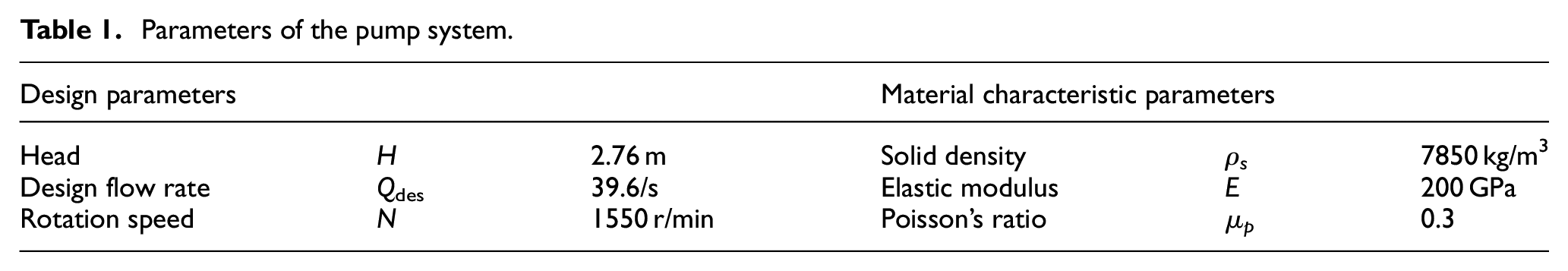
Figure 1 displays a cut-away photograph of the analyzed test pump, which is an axial-flow pump device with a two-way passage. The impeller outer diameter is 300 mm, and the impeller hub diameter is 115 mm. The impeller blade number is 3, and the guide vane blade number is 5. Table 1 lists the material characteristic parameters of the rotor structure and the design parameters of the pump.

Figure 1.

Cut-away photograph of the test pump.

Table 1.

Parameters of the pump system.

Design parameters			Material characteristic parameters
Head	H	2.76 m	Solid density	ρ_s	7850 kg/m³
Design flow rate	Q _des	39.6/s	Elastic modulus	E	200 GPa
Rotation speed	N	1550 r/min	Poisson’s ratio	µ_p	0.3

Governing equations and coupling approach

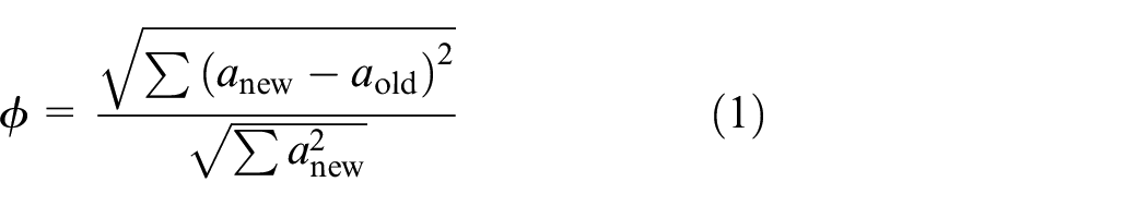
In our study, a fluid part Ω_f and a solid part Ω_s comprised the problem domain Ω, which can both be arbitrary in terms of the shape and the location of the solid and fluid parts. The structural domain Ω_s and the fluid domain Ω_f were separated by the conjoined interface. The fact that the fluid field is formulated and solved on a deforming grid is the essential feature. The deformation of the grid with the structure occurs at the interface, and the grid deformation extends into the fluid field. Figure 2 shows the scheme of the partitioned FSI simulation system. The finite volume method was used initially to compute the flow field, and subsequently, a number of flow parameters were solved. The force load is transferred to the structural dynamic solver through the fluid–structure interface, and these are the boundary conditions for finite element method (FEM) analysis. Therefore, the deformation of the structure can be solved. Next, the FSI calculation convergence is checked considering all the load components that are transferred between the two solvers individually. The FSI calculation will restart from the fluid field simulation if the load that was transferred converges on a specific convergence target for the next time step. Otherwise, the FSI iteration will continue for the current time step. When the convergence of the loads is transferred across the physical interface, the stagger iteration loop will stop. Equation (1) defines the convergence criterion for the load transfer procedure

ϕ = \frac{\sqrt{\sum {(a_{new} - a_{old})}^{2}}}{\sqrt{\sum a_{new}^{2}}}

(1)

where $a_{old}$ represents the load component for the last stagger iteration, $a_{new}$ is the load component transferred in the current stagger iteration, and all individual load component values transferred are summated from different points in space. When $ϕ$ is less than $ϕ_{min}$ , where $ϕ_{min}$ is the convergence target, every quantity can be considered to converge. e indicates the convergence of each quantity transferred across the interface, which is defined by equation (2)

e = \frac{\lg (ϕ / ϕ_{\min})}{\lg (10 / ϕ_{\min})} where 0 < ϕ_{min} < 1

(2)

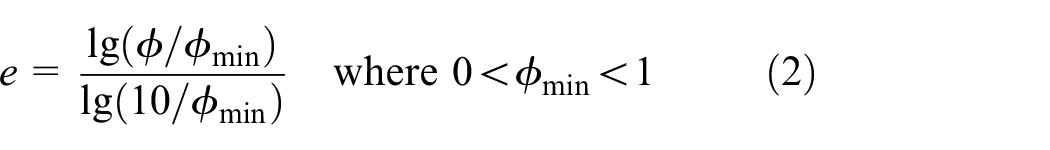
When e reaches a negative value, every quantity will be converged.

Figure 2.

Flowchart of the coupled solution.

Flow is considered to be a viscous, three-dimensional, and unsteady turbulent flow. Therefore, the use of three-dimensional Reynolds-averaged Navier–Stokes questions was assessed. Equations (3) and (4) are for mass conservation and momentum conservation for an incompressible fluid, respectively. Time symbols were excluded since all variables were mean flow quantities

\frac{\partial u_{i}}{\partial x_{i}} = 0

(3)

\frac{\partial}{\partial t} (ρ u_{i}) + \frac{\partial}{\partial x_{j}} (ρ u_{i} u_{j}) = - \frac{\partial p}{\partial x_{i}} + \frac{\partial}{\partial x_{j}} [μ (\frac{\partial u_{i}}{\partial x_{j}} + \frac{\partial u_{j}}{\partial x_{i}}) - \bar{ρ {u^{'}}_{i} {u^{'}}_{j}}] + F_{i}

(4)

where dynamic viscosity is µ, the source item is represented by F_i, and the Reynolds stress is represented by $- ρ \bar{u'_{i} u'_{j}}$ .

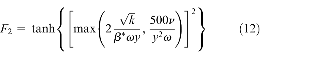
The equations were enclosed with a shear stress transport (SST) turbulence model, and the SST model was a modified $k - ω$ turbulence model. This model is a hybrid of the $k - ε$ and $k - ω$ turbulence models and can automatically switch between main flow and near-wall areas. The following equations are transport equations for k and ω

\frac{\partial (ρ k)}{\partial t} + \frac{\partial (ρ u_{j} k)}{\partial x_{j}} = P_{k} - β^{*} ρ k ω + \frac{\partial}{\partial x_{j}} [(μ + \frac{μ_{t}}{σ_{k 3}}) \frac{\partial k}{\partial x_{j}}]

(5)

\frac{\partial (ρ ω)}{\partial t} + \frac{\partial (ρ u_{j} ω)}{\partial x_{j}} = a_{3} \frac{ω}{k} P_{k} - β_{3} ρ ω^{2} + \frac{\partial}{\partial x_{j}} [(μ + \frac{μ_{t}}{σ_{ϖ 3}}) \frac{\partial ω}{\partial x_{j}}] + 2 (1 - F_{1}) ρ σ_{ϖ 2} \frac{1}{ω} \frac{\partial k}{\partial x_{j}} \frac{\partial ω}{\partial x_{j}}

(6)

P_{k} = μ_{t} (\frac{\partial u_{i}}{\partial x_{j}} + \frac{\partial u_{j}}{\partial x_{i}}) \frac{\partial u_{i}}{\partial x_{j}} - \frac{2}{3} (ρ k + μ_{t} \frac{\partial u_{l}}{\partial x_{l}}) \frac{\partial u_{k}}{\partial x_{k}}

(7)

The following equations are used to calculate the turbulence viscosity

μ_{t} = \frac{ρ a_{1} k}{max (a_{1} ω, S F_{2})}

(8)

S = \sqrt{(\frac{\partial u_{i}}{\partial x_{j}} + \frac{\partial u_{j}}{\partial x_{i}}) \frac{\partial u_{i}}{\partial x_{j}}}

(9)

F_{1} = \tanh {{min [max (\frac{\sqrt{k}}{β^{*} ω y}, \frac{500 ν}{y^{2} ω}), \frac{4 ρ σ_{ω 2} k}{C D_{k ω} y^{2}}]}^{4}}

(10)

C D_{k ω} = max (2 ρ σ_{ω 2} \frac{1}{ω} \frac{\partial k}{\partial x_{j}} \frac{\partial ω}{\partial x_{j}}, 1.0 E^{- 10})

(11)

F_{2} = \tanh {{[max (2 \frac{\sqrt{k}}{β^{*} ω y}, \frac{500 ν}{y^{2} ω})]}^{2}}

(12)

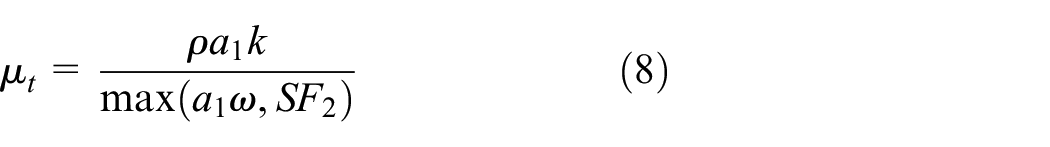
where the coefficients are as follows: $β^{*} = 0.09$ , $a_{1} = 5 / 9$ , $β_{1} = 3 / 40$ , $σ_{k 1} = 2$ , $σ_{ω 1} = 2$ , $a_{2} = 0.44$ , $β_{2} = 0.0828$ , $σ_{k 2} = 1$ , and $σ_{ω 2} = 0.856$ .

The ANSYS code was used for analysis of the impeller that was coupled to the flow calculation for the structure domain. The transient dynamic equation was

M \overset{\cdot\cdot}{q} (t) + C \overset{\cdot}{q} (t) + Kq (t) = Q (t)

(13)

where ${\overset{\cdot\cdot}{q}}_{t} (t)$ means a nodal acceleration vector, ${\overset{\cdot}{q}}_{t} (t)$ a nodal velocity vector, $q_{t} (t)$ a nodal displacement vector, M the structural mass matrix, C the structural damping matrix, K the structural stiffness matrix, and $Q (t)$ the applied load vector. For the time integration of the transient dynamic equilibrium equation, the Hilber–Hughes–Taylor (HHT) method was used. This method is an improved algorithm of the Newmark time integration method. The HHT method is used to solve the transient problem that tries to increase the amount of numerical damping present without degrading the order of accuracy. This is a one-step implicit method. The same Newmark approximations are used in the HHT method. Rayleigh damping is also used in the solving system to apply the damping effect to the transient analysis.

Calculation grids and boundary conditions

Only the pressure is included in the fluid load in the present case. The flow is influenced by the structural deformation by changing the flow geometry. Also, there is no consideration of the influence of the vibration velocity at the moment. The dominant hydrodynamic force component changed slowly, in addition, in comparison to the first rotor natural frequency. A static analysis can be used to determine the structure’s response. It can be assumed that the structure’s response may vary slowly with respect to time. The assumption that only the deflection displacement is considered in the coupled calculations, which were mentioned above, can be seen as acceptable.

The grid generation tool ICEM-CFD 14.5 was used to generate the structured grids for the impeller and guide vane and the unstructured grids for the inlet and outlet passages. Figure 3(a) shows the grids of all the domains partially. Also, the total number of grid nodes for both the stationary and rotating domains was 7,380,888, which was determined by grid independence analysis, as shown in Figure 3(b). There is a second-order of accuracy for the discretization in space. Also, the second-order backward Euler scheme was chosen for time discretization. The interface between the inlet passage and impeller and the guide vane and impeller was set to “transient rotor–stator” to capture the transient rotor–stator interaction in the flow. This was done because the relative position between the impeller and inlet passage with this kind of interface, as well as that between the impeller and guide vane, was changed for each time step. A smooth wall condition was used for the wall function. The chosen time step for the transient simulation was 3.2258 × 10⁻⁴ for the nominal rotating speed. This speed corresponded to a changed angle of Δϕ = 3°. The iteration stopped when the maximum residual was <10⁻⁴ within each time step. To reach the periodically stable results of unsteady flow simulation, 10 revolutions with total time of 0.387096 s have been calculated, and the results were used as the initial boundary for FSI simulation. To make the unsteady FSI results stable, additional six revolutions with total time of 0.232258 s have been calculated.

Figure 3.

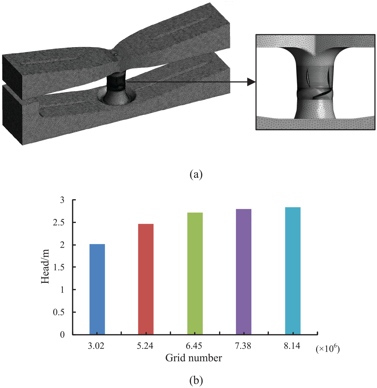
Mesh of the CFD model: (a) grids of all the domains and (b) grid independence analysis.

The FEM model is shown in Figure 4. The fluid–structure interfaces for all wetted surfaces of the blade were defined. The total mesh size of the structure model is 18,540, which was determined by the analysis of the grid independence. The face’s fixed support boundaries are applied to the impeller hub. Figure 5 shows that the hub front and end surfaces were fixed against the axial movement. The cylindrical hub surface was locked against the tangential and radial movements.

Figure 4.

Detailed mesh for impeller.

Figure 5.

Impeller constraints.

As shown in Figure 6, the data are transferred between the fluid and solid domains through a coupling surface. Different interpolation ways have been selected, and the conservative interpolation and the profile preserving interpolation are used for force and deformation transfer, respectively. The under relaxation factor, as an external load transfer parameter, was fixed at 0.75 for all data transferred between the two solvers, and this is an empirical value which has been approved to be an appropriate value for an accurate results.^11,12 This was done to control the solving convergence process. The convergence target for the load transfer was 0.01. Also, the nonmatching area fractions between the structure sides and fluid during the interpolation mapping process for the blade interfaces were <0.4%. This indicated that the two sides of the fluid–structure interface for the load transfer had nearly the same shape, which can make less error for the load transfer. In this article, the time-dependent wall force can be calculated using variable p(t) as follows

F (t) = - \int p (t) n dA

(14)

Figure 6.

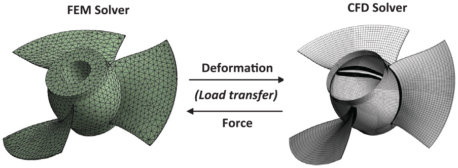
Data interpolation mapping procedure.

To verify the accuracy of the numerical results, the performances of the head versus flow rate were compared between numerical and experimental results. Figure 7 shows that the calculated head is greater than the measurement value, and the calculated head with strong FSI is closer to the measurement value. The calculated heads with and without FSI were both obtained from the average values of unsteady FSI and computational fluid dynamics (CFD) results separately, which have the same initial time and total calculation time. Although small deviations are observed for different flow rates, good agreement is obtained.

Figure 7.

Comparison of numerical and measured Q–H curves.

Results and discussion

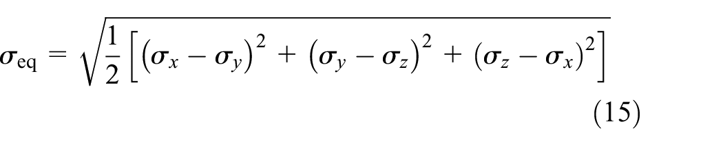
The equivalent stress σ_eq can be calculated by the following equation

σ_{eq} = \sqrt{\frac{1}{2} [{(σ_{x} - σ_{y})}^{2} + {(σ_{y} - σ_{z})}^{2} + {(σ_{z} - σ_{x})}^{2}]}

(15)

Figures 8 and 9 show the maximum equivalent stress and total deformation of the whole structure for different flow rates. The maximum values of the equivalent stress and total deformation decrease with an increasing flow rate and a decreasing head.

Figure 8.

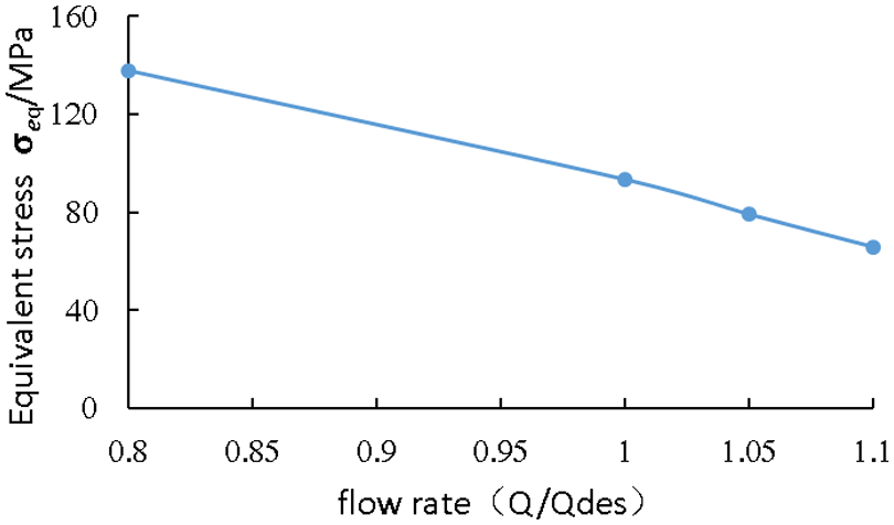
Maximum equivalent stress for different flow rates.

Figure 9.

Maximum total deformation for different flow rates.

Figure 10 shows the distribution of the total deformation on the impeller blade for the four investigated flow rates, which is viewed from the impeller outlet. The total deformation values decrease with an increasing flow rate. Also, the total deformation grows from the hub to the outer diameter. Figure 11 illustrates the equivalent stress distribution on the impeller blade. The higher equivalent stress values can be observed in the area near hub and are quantitatively shown to decrease with an increasing flow rate.

Figure 10.

Distribution of the total deformation on impeller surface.

Figure 11.

Distribution of the equivalent stress on impeller surface.

To study the trend of the total deformation and equivalent stress on the crucial position of the impeller in detail, the wireframe paths are defined in Figure 12. The labels hub-ss, hub-ps, rim-ss, and rim-ps indicate the paths with the direction from the blade trailing edge to leading edge. The leading edge-ps, leading edge-ss, trailing edge-ss, and trailing edge-ps show the paths with the direction from the hub to rim. The short arc paths from the pressure side to suction side are indicated by rim-lr, hub-lr, rim-tr, and hub-tr. In this figure, ps is the pressure side and ss is the suction side.

Figure 12.

Investigated paths on the wireframe.

The distributions of the total deformation on the impeller blade in the examined wireframe paths for the investigated flow rates are shown in Figure 13. The total deformation represents the maximum value among all time steps of each point along the paths. The trend of the total deformation curves remains unchanged for different flow rates, but the values decrease with an increasing flow rate.

Figure 13.

Distribution of the total deformation in the impeller wireframe paths for different flow rates.

Regarding the paths of leading edge and trailing edge, the total deformation increases along the direction from the impeller hub to rim, and in the paths of rim, the deformation decreases from the blade inlet to outlet. In the paths of hub-ps and hub-ss, the total deformation first increases and then decreases, and the peak values of the two paths can be found near a path length of 0.6. In the paths of rim-lr, hub-lr, rim-tr, and hub-tr, the total deformation almost remains unchanged from pressure side to suction side.

The distributions of the equivalent stress on the impeller blade in the wireframe paths for the four flow rates are shown in Figure 14. The equivalent stress is defined as the maximum value among all time steps on each point along the paths. The stress values decrease with an increasing flow rate, and in particular, there is a little difference in the equivalent stress curves under 1.05Q_des and 1.1Q_des because the operating points are quite close.

Figure 14.

Distribution of the equivalent stress in the impeller wireframe paths for different flow rates.

In the paths of rim-ps and rim-ss, the equivalent stress first increases and then decreases dramatically from the trailing edge to leading edge, and the peak values in the two paths can be found near a path length of 0.8. In the paths of hub-ps and hub-ss, the equivalent stress first increases in the path length range of 0–0.65 and then decreases in the range of 0.65–0.88 and finally rises dramatically in the range of 0.88–1.

The peak values of the equivalent stress from the impeller hub to rim can be found in the path length range of 0–0.2. In the paths of leading edge-ps, trailing edge-ss, and trailing edge-ps, the equivalent stress first rapidly increases and then decreases gradually, and in the leading edge-ss, the equivalent stress continues to decrease from the hub to rim.

In the paths of rim-lr and rim-tr, the equivalent stress first decreases and then increases from pressure side to suction side, and the valley values can be seen near path lengths of 0.6 and 0.5. In the hub-tr, the equivalent stress basically remains unchanged except for Q = 0.8Q_des when the equivalent stress fluctuates from 12 to 5 MPa. In the hub-lr, the equivalent stress continues to slightly increase from pressure side to suction side.

Conclusion

A coupled solution of the flow field and structural response of the impeller was established using a two-way coupling method to study the distribution of stress and deformation in the impeller and quantitatively analyze that on the blade along the wireframe paths for different flow rates. The following conclusions can be drawn:

The maximum equivalent stress and maximum total deformation in the impeller are greatly influenced by flow rate, and their values drop with an increasing flow rate and a decreasing head.

The total deformation in the impeller is greater near the blade rim, where the maximum value can be found. The equivalent stress is greater near the blade hub, where the maximum value can be obtained.

The total deformations in the blade rim decrease from blade leading edge to trailing edge, and the total deformations in the paths of leading edge and trailing edge decrease from impeller rim to hub. The equivalent stress in the blade hub initially increases and then declines, and in the end, it rapidly increases from the blade outlet to inlet. In addition, the equivalent stress rises dramatically at first and then descends gradually from the impeller hub to rim.

Because of the loading by complex fluid forces and constraints, the deformation and stress distribution in the impeller cannot be described analytically. However, the knowledge of stress and deformation distribution, especially the field of maximum stress and deformation, is significant for structure design.

Footnotes

Appendix 1

Academic Editor: Mark J Jackson

Declaration of conflicting interests

The author(s) declared no potential conflicts of interest with respect to the research, authorship, and/or publication of this article.

Funding

The author(s) disclosed receipt of the following financial support for the research, authorship, and/or publication of this article: This study was supported by National Science & Technology Pillar Program of China (2015BAD20B01), National Natural Science Foundation of China (grant no. 51409123), Natural Science Foundation of Jiangsu Province (grant no. BK20140554), and China Postdoctoral Science Foundation (grant no. 2015T80507).

References

Tran

Liauzun

Labaste

Methods of fluid–structure coupling in frequency and time domains using linearized aerodynamics for turbomachinery. J Fluid Struct 2003; 17: 1161–1180.

Carstens

Kemme

Schmitt

Coupled simulation of flow-structure interaction in turbomachinery. Aerosp Sci Technol 2003; 7: 298–306.

Campbell

Paterson

EG.

Fluid–structure interaction analysis of flexible turbomachinery. J Fluid Struct 2011; 27: 1376–1391.

Consuegra

Flowers

. Simplified analysis strategies for fluid-structure interaction in high speed turbomachinery. In: ASME 2009 international design engineering technical conferences and computers and information in engineering conference, San Diego, CA, 30 August–2 September 2009, pp.839–843. New York: American Society of Mechanical Engineers.

Schneider

Will

Böhle

. Numerical evaluation of deformation and stress in impellers of multistage pumps by means of fluid structure interaction. In: ASME 2013 fluids engineering division summer meeting, Incline Village, NV, 7–11 July 2013, V01BT10A020 (10 pp.). New York: American Society of Mechanical Engineers.

Benra

Dohmen

. Comparison of pump impeller orbit curves obtained by measurement and FSI simulation. In: ASME 2007 pressure vessels and piping conference, San Antonio, TX, 22–26 July 2007, pp.41–48. New York: American Society of Mechanical Engineers.

Benra

Dohmen

Wan

. Determination of pump impeller deflections: comparison of FSI-simulations to measurements. In: ASME 2006 2nd joint US-European fluids engineering summer meeting collocated with the 14th international conference on nuclear engineering, Miami, FL, 17–20 July 2006, pp.291–296. New York: American Society of Mechanical Engineers.

Erath

Nowotny

Maetz

Modelling the fluid structure interaction produced by a waterhammer during shutdown of high-pressure pumps. Nucl Eng Des 1999; 193: 283–296.

Jiang

Guo

. Numerical calculation on flow field in centrifugal pump based on fluid-structure interaction theorem. Trans Chin Soc Agric Mach 2012; 43: 53–56.

10.

Liu

. Effect of fluid-structure interaction on internal and external characteristics of centrifugal pump. Trans Chin Soc Agric Eng 2012; 28: 82–87.

11.

Pei

Yuan

Dynamic stress analysis of sewage centrifugal pump impeller based on two-way coupling method. Chin J Mech Eng 2014; 27: 369–375.

12.

Pei

Yuan

Fluid-structure coupling effects on periodically transient flow of a single-blade sewage centrifugal pump. J Mech Sci Technol 2013; 27: 2015–2023.

13.

Shi

Zhang

. Structural strength analysis of multistage submersible pump impeller based on fluid-structure interaction. Trans Chin Soc Agric Mach 2013; 44: 70–73.

14.

Luo

Feng

. Cracking reason for Francis turbine blades based on transient fluid structure interaction. Trans Chin Soc Agric Eng 2015; 31: 92–98.

15.

Luo

Zheng

Zhang

Numerical simulation of flow field for axial pump saddle zone based on fluid-structure interaction. J Drain Irrig Mach Eng 2014; 32: 466–471.

16.

Shi

Wang

Zhang

. Stress characteristics in blades of axial-flow pump based on fluid-structure interaction. J Drain Irrig Mach Eng 2013; 31: 737–740.

17.

Zhang

Zheng

Zhang

. Strength analysis of axial-flow pump impeller based on FSI. Appl Mech Mater 2015; 799–800.

Fluid–structure coupling analysis of deformation and stress in impeller of an axial-flow pump with two-way passage

Abstract

Keywords

Introduction

Mathematical model and FSI setup

Pump and system parameters

Governing equations and coupling approach

Calculation grids and boundary conditions

Results and discussion

Conclusion

Footnotes

Appendix 1

Declaration of conflicting interests

Funding

References