Sage Journals: Discover world-class research

Abstract

Searching the lowest-cost path through a graph is central to many problems, including path planning for a mobile robot. By combining Dijkstra’s algorithm, A* algorithm, and rolling window principle, a new rapid path planning algorithm for a mobile robot in dynamic environment is proposed. First, Dijkstra’s algorithm is applied to find an initial path from the initial state to the goal. As a robot moves along the path, if a possible collision is predicted, a local optimal target state within the detection range of the sensors is selected using the rolling window principle. Then, an optimal path from the robot’s current location to this local target is searched through A* algorithm and a new path which leads the robot to move from current location to the goal is obtained. Compared to other algorithms, such as ant colony optimization algorithm, A* algorithm, and D* algorithm, the proposed algorithm can always find an optimal path during re-planning and at the meantime greatly reduce the re-planning time. The simulation results prove the feasibility and effectiveness of the proposed algorithm.

Keywords

Path planning dynamic environment Dijkstra’s algorithm A* algorithm rolling window

Introduction

Path planning for mobile robot, which is an important content in the field of intelligent robot research, is typically stated as finding a sequence of state transitions for the robot from its initial state to some desired goal state. The path is optimal if the sum of the transition costs is minimal across all possible sequences through the map.

Up to now, there have been many researches about path planning of mobile robot in a static environment.^1–13 However, the real environment in which robot works is usually dynamic and there are some unknown moving obstacles in it. As a result, any path generated using static environment information may turn out to be invalid if the robot detects moving obstacles by its equipped sensors. Thus, it is important that the robot is able to efficiently re-plan optimal paths when a moving obstacle appears. There exist a number of algorithms for performing this re-planning. Hao et al.¹⁴ apply the polar coordination particle swarm optimization (PPSO) algorithm to search for a global optimal path based on the static obstacle information, when the robot moves along the path, an online real-time path planning strategy is adopted to avoid dynamic obstacles by means of predicting the future positions of moving obstacles. Li et al.¹⁵ present an improved artificial potential field algorithm-based simultaneous forward search method for autonomous mobile robot path planning in partially known, unknown, and dynamic complex environments. Mobadersany et al.¹⁶ present a fuzzy path planning method to navigate a robot among unknown moving obstacles in complex environments. Other algorithms including hierarchical reinforcement learning method,¹⁷ ant colony optimization (ACO),^18,19 multi-artificial fish-swarm algorithm,²⁰ and so on sometimes can be applied to solve the problems of path planning for mobile robot in dynamic environments, but they are suboptimal or inefficient, particularly in complex environments where the goal is far away and large numbers of moving obstacles exist.

Dijkstra’s algorithm and A* algorithm are mainly used for path planning in known environment, and rolling window principle is used for obstacle avoidance in unknown environment. Based on the three methods, this article innovatively presents a collision prediction method and a local target selection method, and then a high efficient algorithm for generating optimal paths for mobile robot in a complex dynamic environment is proposed. The new algorithm can always find an optimal path from the robot’s current location to the goal by local re-planning.

The rest of the article is organized as follows. The second section introduces the environment model of the algorithm. The third section briefly reviews the Dijkstra’s algorithm and A* algorithm. The fourth section presents the new path planning algorithm in detail. The fifth section introduces and evaluates the comparison of the new algorithm with other three algorithms. Finally, the last section gives the conclusions and suggestions.

Environment model

As both Dijkstra and A* are grid traversal search algorithms, we should first establish the grid model of the environment map by the grid method. The grid method is to divide the map into some adjacent grids with the same size. The size of the grid is determined by the size of the mobile robot, and it affects the efficiency and searching precision of algorithm. The grid model of an environment map is as shown in Figure 1.

Figure 1.

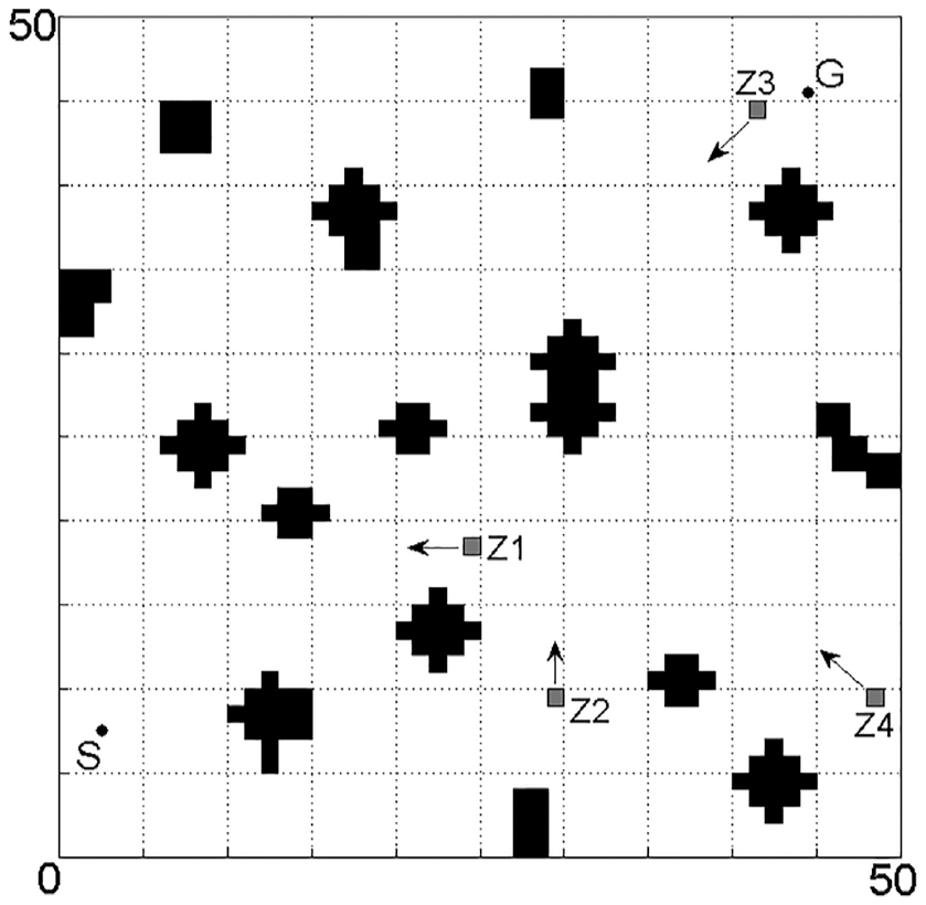
Environment model.

Figure 1 represents the square with a side of length 50 m, it is divided into a 50 × 50 grid of cells. Each cell represents a state and is connected to its eight neighbors. The black regions are known static obstacle locations, while the white regions are locations known to be in free space. The four small gray squares, respectively, denoted by Z1, Z2, Z3, and Z4, are unknown moving obstacles, they will move, respectively, along the direction of the arrows next to them until they collide with the static obstacles or the boundary of the map. The static obstacles are stored in the map, but the moving obstacles are not. The position coordinates of the initial state, S, are (3, 8) and the position coordinates of the goal state, G, are (45, 46). The task of robot path planning is to find an optimal path that leads the robot from S to G.

The robot is able to move freely on the obstacle-free grids. The parameter ε is defined to be step length, which is the distance between the current grid where the robot stands and the next target grid. The robot can only choose its adjacent grid as the next target grid, such that ε = 1 m if the robot moves along vertical and horizontal directions, and ε = m if the robot moves along diagonal directions. The proposed algorithm lays out a global optimal path based on the static obstacle information at first, and then the robot starts at state S and follows the optimal path to the goal state G, with some range sensors and velocity sensors detecting the distance between obstacles and the robot. If at some location, the sensors detect a moving obstacle, the algorithm would predict the collision between the robot and the moving obstacle according to the position, speed and moving direction of the moving obstacle, and an online real-time path re-planning strategy would be adopted to avoid the collision.

Dijkstra’s algorithm and A* algorithm

In order to improve the efficiency of planning, an optimal collision-free path for a mobile robot in the re-planning process, Dijkstra’s algorithm is adopted to pre-process the static environment map data, which plans and saves optimal paths from the goal, G, to all free states. As the robot moves toward the goal, if it is about to collide with a moving obstacle, a local optimal state is chosen as the next target state based on rolling window principle, and then A* algorithm is adopted to re-plan a local optimal path from the robot’s location to the local target. The new path can guide the robot to avoid obstacles. The proposed algorithm combines Dijkstra’s algorithm and A* algorithm in order to describe the new algorithm clearly the principles of the two algorithms are illustrated briefly in the following.

Dijkstra’s algorithm

The main idea of Dijkstra’s algorithm is to expand outward from the goal state G, compute optimal path costs from G to all other free states, and store optimal path from each state to G until all states have been traversed. In order to ensure the safety of a robot, it is necessary to keep the robot at a safe distance away from obstacles. That is to say, only if the distance between a state and the nearest obstacle is no less than the safe distance can the state be traversed so that the planned path is safe.

Dijkstra’s algorithm maintains an OPEN list of states for expansion. The OPEN list is used to store states waiting to be traversed. Every state X except G has a hidden arrow points to a next state Y denoted by p(X) = Y. Dijkstra’s algorithm uses the arrows to represent paths to the goal. Every state X has an associated tag t(X), such that t(X) = new if X has never been on the OPEN list, t(X) = open if X is currently on the OPEN list, and t(X) = closed if X is no longer on the OPEN list. The cost of moving from X to a neighboring state Y is a positive number given by the moving cost function c(X, Y). The sum of the moving costs from X to G is given by the path cost function g(X). The procedure of Dijkstra’s algorithm is given below.

Function: Dijkstra (S, G)
01) for each state X in the environment model: 02) t(X) = new; 03) Initialize the OPEN list to be empty; Place state G on the OPEN list; t(G) = open; g(G) = 0; 04) while OPEN≠NULL: 05) Find the state, X, on the OPEN list with minimum path cost; 06) for each neighbor Y of X: 07) if Y is not next to an obstacle 08) if t(Y) = new 09) p(Y) = X; g(Y) = g(X)+c(X, Y); Place Y on the OPEN list; t(Y) = open; 10) else if t(Y) = open 11) if g(X)+c(X, Y)<g(Y) 12) g(Y) = g(X)+c(X, Y); p(Y) = X; 13) Delete X from the OPEN list; t(X) = closed; 14) if t(S)≠closed 15) return NO-PATH; 16) The optimal path for S can be discovered by following the arrows toward the goal.

Function: Dijkstra (S, G)

01) for each state X in the environment model:
02) t(X) = new;
03) Initialize the OPEN list to be empty; Place state G on the OPEN list; t(G) = open; g(G) = 0;
04) while OPEN≠NULL:
05) Find the state, X, on the OPEN list with minimum path cost;
06) for each neighbor Y of X:
07) if Y is not next to an obstacle
08) if t(Y) = new
09) p(Y) = X; g(Y) = g(X)+c(X, Y); Place Y on the OPEN list; t(Y) = open;
10) else if t(Y) = open
11) if g(X)+c(X, Y)<g(Y)
12) g(Y) = g(X)+c(X, Y); p(Y) = X;
13) Delete X from the OPEN list; t(X) = closed;
14) if t(S)≠closed
15) return NO-PATH;
16) The optimal path for S can be discovered by following the arrows toward the goal.

Figure 2 shows an optimal path from S to G, which is obtained by the simulation of Dijkstra’s algorithm.

Figure 2.

Offline optimal path.

It can be seen from Figure 2 that the path keeps a certain distance away from the obstacles, which protects the safety of the robot.

As seen above, Dijkstra’s algorithm can compute optimal path costs from the goal state to all other free states. These data can be efficiently utilized in the real-time path re-planning process.

A* algorithm

In the process of state expansion, Dijkstra’s algorithm does not directly expansion toward the initial state. Rather, the sole consideration in determining the next expansion state is its distance from the goal state. The algorithm therefore expands outward from the goal state aimlessly. Unlike Dijkstra, the A* algorithm introduces heuristic information into the path cost function to define a new function, the estimated path cost function, to focus the expansion on the direction of the initial state and reduce the total number of state expansions.

The estimated path cost function of A* is defined as follows

f (X) = g (X) + h (X)

(1)

where f(X) denotes the estimated path cost from S through X to G, g(X) denotes the actual path cost from X to G, and h(X) is the heuristic function which denotes the estimated path cost from S to X. The heuristic function is generally expressed as Manhattan distance, diagonal distance, or Euclidean distance. This article adopts diagonal distance as the estimated path cost. After calling the A* algorithm A*(S, G), an optimal path for state S can also be discovered by following the arrows toward the goal.

The rapid path planning algorithm

Algorithm description

The flow diagram of the rapid path planning algorithm is as shown in Figure 3.

Figure 3.

Flow diagram of the rapid path planning algorithm.

This rapid path planning algorithm first adopts Dijkstra’s algorithm to plan optimal paths from the goal state to all obstacle-free states. The robot then starts at the initial state and moves along the optimal path until it either reaches the goal or detects a moving obstacle. Once a moving obstacle is detected, the collision prediction function is immediately called to predict whether the robot will collide with the moving obstacle. If a collision were to occur, the local target selection function is called to search a local optimal target state L, and A* algorithm is adopted to plan a local optimal collision-free path from the current location of the robot to L. As the optimal path from L to G is known, the robot continues to move along the optimal path from the current location through L to G.

The collision prediction function

The task of the collision prediction function is to predict whether the robot will collide with moving obstacles, so as to decide whether an obstacle avoidance process is necessary.

The robot is equipped with range sensors and velocity sensors; the detection radius of the sensors is denoted by r, which is bigger than step length ε. At any time t, the detection range of the sensors is a circular area with the location of the robot as the center and r as the radius, which is denoted by D_R(t). The sensors can detect the position, speed, and moving direction of each moving obstacle in the detection range. Let v_o denote the speed of the moving obstacle, and v and T denote the speed and the control cycle of the robot. To guarantee the safety of the robot, these parameters should satisfy the equation

(v + v_{o}) \times T < r

(2)

which means that in a control cycle, the maximum relative displacement between the robot and the moving obstacle must be less than the detection radius of the sensors. Because T = ε/v, we obtain

v_{o} < (\frac{r}{ε} - 1) v

(3)

Therefore, the collision prediction function can timely predict the collision between the robot and moving obstacle only if v_o fulfills formula (3).

At any moment, we are only fully aware of the environment information within the detection range of the robot’s sensors; therefore, only the collisions that would occur in the detection range can be predicted. Assuming that the sensors detect one or more moving obstacles when the robot moves to location R at time t, then the collision prediction function is called and its pseudocode is given below. The parameter, C_ollision, denotes the tag of collision, C_ollision = 0 if the robot would not collide with the moving obstacles, otherwise, C_ollision = 1. The embedded routine, POS, returns a new location where the moving obstacle will reach in one control cycle of the robot.

Function: collision-prediction (R)
01) Get the location O_X, speed v_oX and moving direction D_X of each moving obstacle X in D_R(t); Define a variable O_1X for each X and let O_1X = O_X; Initialize C_ollision to zero; R₁ = p(R); 02) while R₁ ∈ D_R(t) 03) Compute the travel time, δt, of the robot in the next movement process; 04) for each moving obstacle X: 05) O_2X = POS(O_1X, v_oX, D_X, δt); 06) if the minimum distance of location R₁ to the points on line segment O₁_XO_2X is less than the safe distance 07) C_ollision = 1; return C_ollision; 08) else 09) O_1X = O_2X; 10) R₁ = p(R₁); 11) return C_ollision.

Function: collision-prediction (R)

01) Get the location O_X, speed v_oX and moving direction D_X of each moving obstacle X in D_R(t); Define a variable O_1X for each X and let O_1X = O_X; Initialize C_ollision to zero; R₁ = p(R);
02) while R₁ ∈ D_R(t)
03) Compute the travel time, δt, of the robot in the next movement process;
04) for each moving obstacle X:
05) O_2X = POS(O_1X, v_oX, D_X, δt);
06) if the minimum distance of location R₁ to the points on line segment O₁_XO_2X is less than the safe distance
07) C_ollision = 1; return C_ollision;
08) else
09) O_1X = O_2X;
10) R₁ = p(R₁);
11) return C_ollision.

If the robot will not collide with the moving obstacle, it continues to move along the old path. Otherwise, the local target selection function is called to search a local optimal target state so as to re-plan a local optimal path for avoiding collision.

The local target selection function

When a possible collision between the robot and a moving obstacle is predicted, a global path planning method could be used to re-plan a new path from the current location of the robot to the goal state, but this is inefficient if the environment is large and/or the goal is far away. On the other hand, if a state, which is far away from the moving obstacle, is randomly selected as the local target of path re-planning, the new path could guide the robot to avoid the obstacle, but the cost of the new path may not be optimal. As a result, there is a need to select an appropriate local target state to ensure the efficiency and performance of the algorithm.

To solve the path planning problem of mobile robot in dynamic environment, Xi and Zhang²¹ present a new method, which is based on the rolling window principle of predictive control algorithm to plan paths for a mobile robot. They place certain restrictions on the environment model to make sure the new method can find a path. In addition, in the method, the state that is nearest to the goal in the observation window area is selected as a local target; thus, it usually cannot get the global optimal solution. As all the shortest paths from the goal state to any obstacle-free state are found by Dijkstra’s algorithm, the rolling window principle described in Xi and Zhang²¹ can be used to search the local optimal target state in the observation window area, through which the robot can move along the optimal path from the current location to the goal.

The observation window model

The observation window area of a robot is namely the detection area of the robot’s sensors. Assume the robot’s sensors detect a moving obstacle at time t, the observation window model of this moment is shown in Figure 4. Both the robot and the moving obstacle are regarded to be point-sized and assuming that they move at constant velocities. In Figure 4, R denotes the current location of the robot, whose moving speed is denoted by v, and the moving direction of the robot is uncertain. The circular area, which is denoted by D_R(t), represents the detection range of the robot’s sensors, its radius is denoted by r. Point O and point A are both on the circle and O represents the location of the moving obstacle which is moving along OA at a speed of v_o. The black area represents known obstacle and is stored in the map. Assuming that the robot will collide with the moving obstacle at point C; RC represents the path of the robot and OC represents the path of the moving obstacle, the lengths of the two paths are, respectively, denoted by d and d_o. B is a point on line segment OA, and RB is perpendicular to OA.

Figure 4.

Observation window model.

Definition 1: entry angle

Entry angle, which is denoted by α, is defined as the angle between the moving direction of a moving obstacle and the line from the obstacle to the robot when the obstacle enters the observation window area of the robot. As shown in Figure 4, α = ∠ROA. Obviously, when a moving obstacle moves to the boundary of the observation window area D_R(t), the robot could collide with the obstacle in D_R(t) only if 0 ≤ α < π/2.

A collision happens when the robot and the moving obstacle reach the same location at the same time. We thus have

\frac{d}{v} = \frac{d_{o}}{v_{o}}

(4)

where rsin α ≤ d ≤ r and 0 < d_o ≤ 2rcosα. According to the geometrical relationship of triangle, d, d_o, r and α fulfill the equations

{\begin{matrix} d = \sqrt{B C^{2} + R B^{2}} \\ BC = | d_{o} - r \cdot \cos α | \\ RB = r \cdot \sin α \end{matrix}

(5)

wherever the point C is on the line segment OA (except the point O). According to equations (4) and (5), we obtain

(v_{o}^{2} - v^{2}) d_{o}^{2} - 2 {rv}_{o}^{2} \cos α \cdot d_{o} + r^{2} v_{o}^{2} = 0

(6)

which is a quadratic equation about d_o. The solution of the equation is

d_{o} = \frac{2 {rv}_{o}^{2} \cos α \pm \sqrt{Δ}}{2 (v_{o}^{2} - v^{2})}

(7)

where

Δ = 4 r^{2} v_{o}^{2} (v^{2} - v_{o}^{2} si n^{2} α)

(8)

As shown in Figure 4, if a collision between the robot and the moving obstacle is sure to happen, then it must occur on the line segment OR if α = 0; and if α > 0, the collision must occur on OA. When α > 0, if Δ < 0 (namely v < v_o sinα), then equation (6) has no real root; if Δ = 0 (namely v = v_o sinα), then equation (6) has one real root which is d_o = r/cosα; if Δ > 0 (namely v > v_o sinα), then equation (6) has two real roots. The solution of the equation represents the position where the robot would collide with the moving obstacle.

Definition 2: restricted area

In order to ensure the safety of the robot, we connect the current location of the moving obstacle and the predicted collision point with a line segment (represented by OC in Figure 4), and define the area, which consists of the states on the line segment, as restricted area that forbidden to pass.

According to the researches and analysis above, the possible collision point between the robot and the moving obstacle is not unique. Therefore, when a collision is predicted, each state on OA is examined to ensure it may not be a possible collision point if the robot moves along a shortest path toward it so that all the possible collision points can be found and a complete restricted area can be established. If there are multiple moving obstacles within the observation window area, we will have to, respectively, establish the restricted area for each moving obstacle.

Definition 3: escape boundary

For any state X in the observation window area, if all states on the line segment XR are obstacle-free states, then X is called a visible state. All visible states constitute a visible area; and all accessible states, which are not next to obstacles or restricted areas, on the boundary of visible area constitute an escape boundary. The visible area model of the observation window is shown in Figure 5.

Figure 5.

Visible area model.

In Figure 5, the thick solid line OC represents the restricted area, the gray-shaded area represents the visible area, and the thin solid lines on the boundary of the visible area constitute the escape boundary. At this moment, the optimal path from the robot’s current location to the goal is certain to cross the escape boundary; and the state, at which the intersection point locates, is found and selected as the local optimal target.

Implementation of the local target selection function

According to the rolling window principle, once the robot takes a step, a local optimal target is found based on the local environment information of the observation window area, and an optimal path from the robot’s current location to the local target is planned. It is obvious that if every local target is on the current global optimal path, then we can say the complete path of the robot from the initial state to the goal is globally optimal.

Let E_B list denote the set of states of the escape boundary. For each state X on the E_B list, the estimated cost of the path from the robot’s current location R through X to G, which is denoted by f(R, X), is defined as follows

f (R, X) = g (X) + h (R, X)

(9)

where g(X) denotes the minimum path cost from X to G, and h(R, X) denotes the estimated path cost from R to X. And because state X is visible to R, h(R, X) is equal to the minimum path cost from R to X; therefore, f(R, X) is equal to the minimum path cost from R through X to G. As a result, we can know that if a state Y on the E_B list fulfills the equation

f (R, Y) = \min {f (R, X) | X \in E_{B}}

(10)

then Y is the current local optimal target state. If several states are possible, it is sufficient to choose any one of them.

Suppose the observation window model is established as shown in Figure 4, then the pseudocode of the local target selection function is given below.

Function: local-target-selection (R)
01) for each moving obstacle, which is located at O, in D_R(t): 02) for each state X on the line segment OA: 03) if X is an obstacle-free state 04) Assuming that both the robot and the moving obstacle move toward X, compute the shortest distance δd between the robot and the obstacle in the moving process until any of them reaches X; 05) if δd is less than the safe distance which is pre-established 06) Mark X as a possible collision state; 07) else 08) break; 09) Connect O and the possible collision state, which is located farthest from it, with a line segment, and all the states on the line segment constitute a restricted area; 10) Initialize the E_B list to be empty; 11) for each state X on the boundary of D_R(t): 12) if all states on the line segment XR are free states 13) if all neighboring states of the states on XR are free states 14) Place X on the E_B list; 15) else 16) Traverse all the states on XR, select a state, which is next to an obstacle state or restricted state and located farthest from X, and denote the state by Y; Place all the states on XY on the E_B list; 17) for each state X on the E_B list: 18) f(R, X) = g(X) + h(R, X); 19) return the state on E_B with minimum f(R, X) value.

Function: local-target-selection (R)

01) for each moving obstacle, which is located at O, in D_R(t):
02) for each state X on the line segment OA:
03) if X is an obstacle-free state
04) Assuming that both the robot and the moving obstacle move toward X, compute the shortest distance δd between the robot and the obstacle in the moving process until any of them reaches X;
05) if δd is less than the safe distance which is pre-established
06) Mark X as a possible collision state;
07) else
08) break;
09) Connect O and the possible collision state, which is located farthest from it, with a line segment, and all the states on the line segment constitute a restricted area;
10) Initialize the E_B list to be empty;
11) for each state X on the boundary of D_R(t):
12) if all states on the line segment XR are free states
13) if all neighboring states of the states on XR are free states
14) Place X on the E_B list;
15) else
16) Traverse all the states on XR, select a state, which is next to an obstacle state or restricted state and located farthest from X, and denote the state by Y; Place all the states on XY on the E_B list;
17) for each state X on the E_B list:
18) f(R, X) = g(X) + h(R, X);
19) return the state on E_B with minimum f(R, X) value.

If a local optimal target state is denoted by L, then the new path is supposed to be from the robot’s current location through L to G. However, if the hidden arrow of L points to an obstacle state or restricted state, the path is not feasible. Figure 6 shows an example.

Figure 6.

An example of local optimal target.

In Figure 6, R and O, respectively, represent the locations of the robot and moving obstacle, and the gray-shaded grid, which is denoted by C, represents the predicted collision state. The thin solid lines constitute the escape boundary. If the gray-shaded grid D is the local optimal target state and p(D) = C, then the robot cannot avoid collision with the moving obstacle if it moves from the current location through D to G.

In this case, the obtained local optimal target state on the escape boundary is unavailable; thus, it is necessary to choose a new local target state for the robot. As the optimal path from R to G must pass through one of R’s neighbors, and the robot moves one cell at a time, we can select the local optimal target state from all the neighboring states of R. In order to keep the robot from moving along the old path, the state on the old path should not be selected. As shown in Figure 6, the candidate neighboring states of R are marked as triangles.

For each available neighboring state X of R, compute the estimated path cost from R through X to G by equation (9), select the one with the minimum path cost value as the local optimal target.

Algorithm procedure

The procedure of the rapid path planning algorithm is given below.

Algorithm: rapid-path-planning (S, G)
01) Convert the environment to a grid map; Input the speed v of the robot; 02) Dijkstra (S, G); 03) R = S; 04) while R ≠ G: 05) if some moving obstacles are detected within the detection range 06) C_ollision = collision-prediction (R); 07) if C_ollision = 1 08) L = local-target-selection (R); 09) L₁ = p(L); 10) if L₁ is a free state 11) A(R, L); 12) else 13) for each accessible neighboring state X of R (except p(R)): 14) f(R, X) = g(X) + h(R, X); 15) Search the state, L_N, with minimum f(R, X) value from all the candidate neighboring states of R; p(R) = L_N; 16) R = p(R); 17) return GOAL-REACHED*.

Algorithm: rapid-path-planning (S, G)

01) Convert the environment to a grid map; Input the speed v of the robot;
02) Dijkstra (S, G);
03) R = S;
04) while R ≠ G:
05) if some moving obstacles are detected within the detection range
06) C_ollision = collision-prediction (R);
07) if C_ollision = 1
08) L = local-target-selection (R);
09) L₁ = p(L);
10) if L₁ is a free state
11) A*(R, L);
12) else
13) for each accessible neighboring state X of R (except p(R)):
14) f(R, X) = g(X) + h(R, X);
15) Search the state, L_N, with minimum f(R, X) value from all the candidate neighboring states of R; p(R) = L_N;
16) R = p(R);
17) return GOAL-REACHED.

Algorithm simulations and analyses

Simulations

Figure 7 illustrates the operation of the rapid path planning algorithm for a mobile robot path planning problem in a dynamic environment. All of the moving obstacles, denoted by Z1, Z2, Z3, and Z4, are unknown before the robot starts its traverse. The robot moves at a constant speed of 1 m/s, and the detection range of the sensors equipped on the robot is a circle with the radius of 7 m. The moving obstacles move 0.5 m/s. When the moving obstacles collide with static obstacles, they will change their directions.

Figure 7.

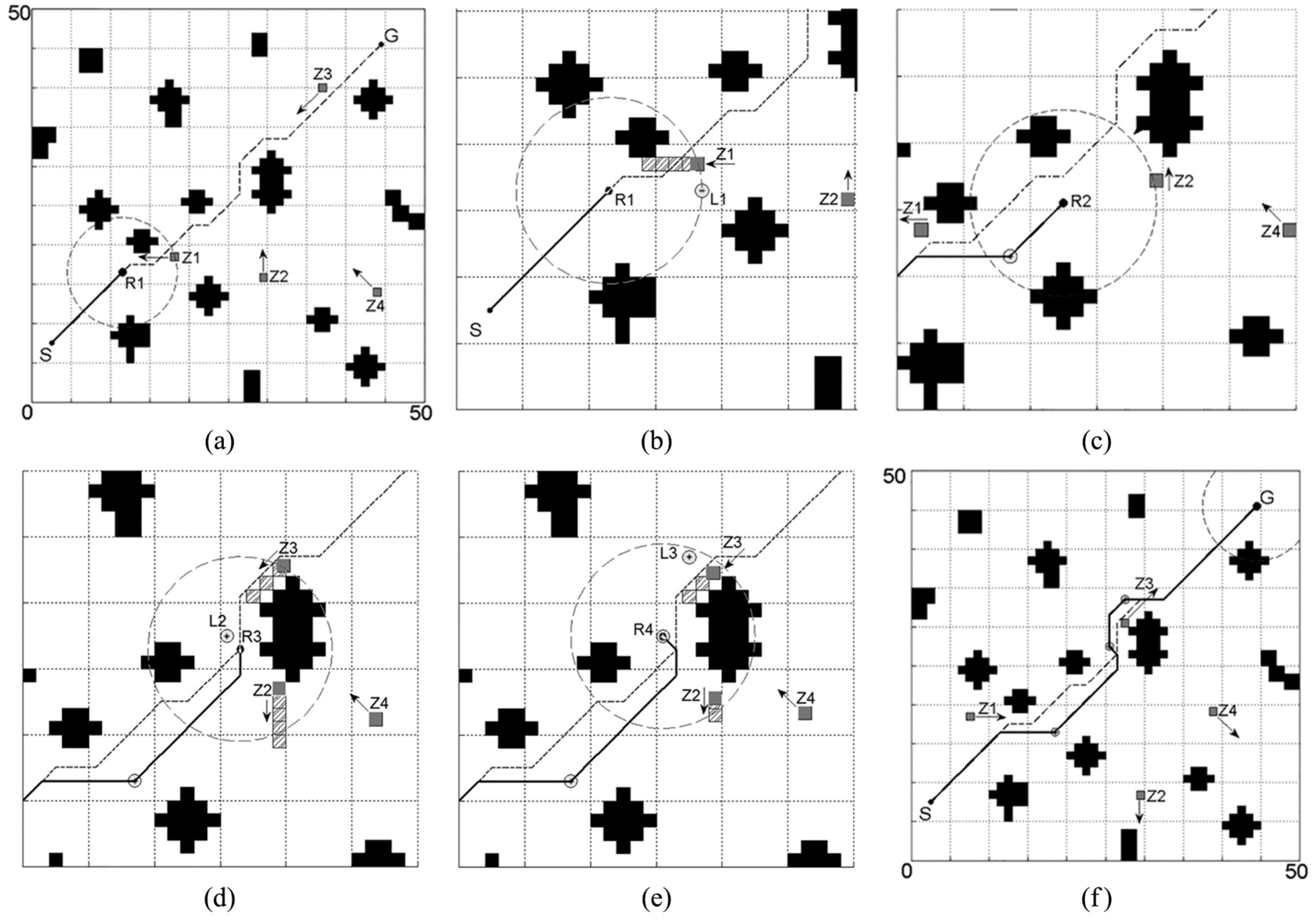
The moving process of a robot: (a) The moving obstacle Z1 is detected, (b) The local optimal target state L1 is searched out, (c) The moving obstacle Z2 is detected, (d) The moving obstacle Z3 is detected and then the local optimal target state L2 is searched out, (e) The local optimal target state L3 is searched out, and (f) The robot reaches the goal state.

The robot starts at state S and begins following the optimal path, which is planned using Dijkstra’s algorithm, to state G. At state R1, the robot’s sensors detect the moving obstacle Z1, as shown in Figure 7(a), where the solid line indicates the path that the robot has traversed, the dotted circle indicates the detection range of the robot’s sensors, and the arrows indicate the moving directions of the moving obstacles. Then, a possible collision between the robot and Z1 is predicted using the collision prediction function, and therefore the local target selection function is called to search a local optimal target state. As Figure 7(b) shows, the area filled with slant lines indicates a restricted area, and the state L1 indicates the local optimal target state. An optimal path from R1 to L1 is planned using A* algorithm, and then the robot moves along the new path from R1 through L1 to G. When the robot moves to state R2, its sensors detect Z2, as shown in Figure 7(c).

It is predicted that the robot would not collide with Z2, so it continues to move along the old path and when it moves to state R3, the moving obstacle Z3 is detected, as shown in Figure 7(d). At this moment, there are two moving obstacles, Z2 and Z3, within the detection range of the robot’s sensors. It is predicted that the robot would collide with Z3; thus, a local optimal target state, which is denoted by L2, is selected for the obstacle avoidance.

Move the robot to state L2, which is denoted by R4 in Figure 7(e), then the collision prediction function and local target selection function are called again and the state L3 is selected as a new local optimal target state. Finally, an optimal path from R4 to L3 is planned using A* algorithm and the robot reaches the goal along the path from R4 through L3 to G, as shown in Figure 7(f).

Figure 7 illustrates the whole process of planning and control of a robot. The simulation results show that when a robot moves in a dynamic environment, the proposed algorithm can guide the robot to plan a new path to avoid the moving obstacles and reach the goal state successfully.

Experimental comparisons and analyses

The simulation experiment described in the last section proves the feasibility of the algorithm proposed in this article. In order to verify the efficiency of the algorithm, ACO algorithm, A* algorithm, and D* algorithm are applied in the same simulation environment as the last section.

ACO algorithm has been widely concerned and applied because of its advantages such as positive feedback, strong robustness, and easy combining with other algorithms. This article adopts an improved ACO algorithm presented in Liu et al.¹⁸ to take path planning experiment. In the movement process of a robot, as long as a possible collision between the robot and a moving obstacle is predicted, the algorithm chooses a state on the old path as a local target and plans an optimal path from the robot’s current location to the local target state. Then, the robot moves along the new path from the robot’s current location through the local target state to the goal state. The parameters configuration of the ACO is shown in Table 1, where K indicates the largest number of iterations, M indicates the total number of ants, α and β, respectively, indicate the stimulating factors of pheromone concentration and visibility, ρ indicates the coefficient of the pheromone volatilization, Q indicates the initial value of the pheromone concentration, and N indicates the distance of the chosen local target state from the predicted collision point. The simulation results are shown in Figure 8, where the dotted line represents the initial path and the solid line represents the actual path through which the robot has passed.

Table 1.

Parameters configuration of ant colony algorithm.

Category	Parameters
Category		K	M	α	β	ρ	Q	N
Global planning	20	20	1	3	0.3	80	–
Local planning	15	15	1	5	0.4	15	4

Figure 8.

Simulation results of the ant colony optimization.

When A* algorithm is used to solve the path planning problem of mobile robot in dynamic environment, it will search an optimal path from the current location of the robot to the goal as long as the robot’s sensors detect a moving obstacle and a possible collision between the robot and the moving obstacle is predicted. The simulation results are shown in Figure 9.

Figure 9.

Simulation results of A* algorithm.

D* algorithm¹³ is often used to solve the path planning problem of mobile robot in partially known or totally unknown static environment. However, the dynamic problem can be solved by breaking it up into a series of static problems; thus, D* is also feasible to solve the path planning problem of mobile robot in dynamic environment. The simulation results of D* algorithm are shown in Figure 10.

Figure 10.

Simulation results of D* algorithm.

The simulation results show that all the four algorithms can guide the robot to avoid moving obstacles and reach the target state. Characteristics of the paths calculated by the four algorithms are shown in Table 2, where pre-processing time indicates the time taken to plan initial path, and average time of re-planning indicates the average time from predicting a collision to getting a new path.

Table 2.

Performance comparison of the four algorithms.

Parameter	ACO	A*	D*	Rapid path planning
Path length (m)	64.4	62.4	63.3	63.3
Pre-processing time (ms)	1304	48	163	135
Re-planning times	2	2	2	3
Average time of re-planning (ms)	232	42	32	3

Since the initial paths calculated by the four algorithms are different, the robot may detect a moving obstacle in different time and location when using different algorithms to avoid obstacles; therefore, the actual paths through which the robot moves to the goal are different. As shown in Table 2, the path computed by the rapid path planning algorithm is shorter than that by ACO for approximately 1.7%, but longer than that by A* algorithm for approximately 1.4% and equal to that by D* algorithm.

Compared with the other three algorithms, ACO increases the pre-processing time by 7.0–26.2 times and the average re-planning time by 4.5–76.3 times, which show that it is the least efficient. The efficiency of ACO is associated with its time complexity, which is expressed as

T (n) = O (N_{c} \times m \times n^{2})

(11)

where N_c indicates the largest number of iterations, m indicates the total number of ants, and n indicates the number of obstacle-free states. If N_c and m are small, the algorithm may fail to find the optimal solution. But if N_c and m become large, the computing time of the algorithm will increase.

It is different from A* algorithm that the rapid path planning algorithm traverses all of the obstacle-free states when planning the initial path; thus, the pre-processing time of the rapid path planning algorithm is 2.8 times that of A* algorithm. And in the re-planning process, the rapid path planning algorithm only plans a local path but A* algorithm needs to plan a global path; thus, the average re-planning time of the rapid path planning algorithm decreases by 92.9%. Compared to D* algorithm, the rapid path planning algorithm decreases the pre-processing time by 17.2% and the average re-planning time by 90.6%, which are consistent with the expectations.

Experiments in complex environment and analysis

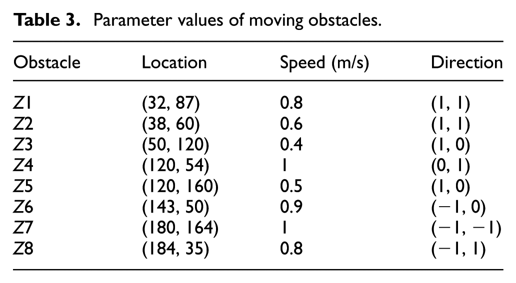
The four algorithms above are tested in a complex environment to verify optimality. Figure 11 shows an environment model of 200 m×200 m. The known static obstacles are shown in black and the unknown moving obstacles are shown in gray. The robot moves at a constant speed of 1 m/s, and the detection range of sensors is a circle with the radius of 7 m. The locations, speeds, and directions of the eight moving obstacles are given in Table 3.

Figure 11.

Complex environment model.

Table 3.

Parameter values of moving obstacles.

Obstacle	Location	Speed (m/s)	Direction
Z1	(32, 87)	0.8	(1, 1)
Z2	(38, 60)	0.6	(1, 1)
Z3	(50, 120)	0.4	(1, 0)
Z4	(120, 54)	1	(0, 1)
Z5	(120, 160)	0.5	(1, 0)
Z6	(143, 50)	0.9	(−1, 0)
Z7	(180, 164)	1	(−1, −1)
Z8	(184, 35)	0.8	(−1, 1)

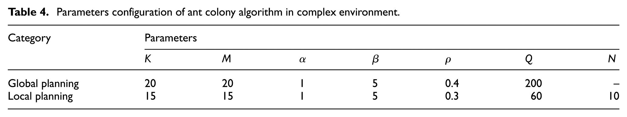
We conduct three simulation experiments for each algorithm in the same environment. In experiment 1, the coordinates of initial state and goal state are (8, 12) and (190, 180); in experiment 2, the coordinates of initial state and goal state are (18, 188) and (185, 35); in experiment 3, the coordinates of initial state and goal state are (180, 183) and (6, 30). The parameters configuration of ant colony algorithm is shown in Table 4.

Table 4.

Parameters configuration of ant colony algorithm in complex environment.

Category	Parameters
Category	K	M	α	β	ρ	Q	N
Global planning	20	20	1	5	0.4	200	–
Local planning	15	15	1	5	0.3	60	10

The simulation results are shown in Table 5. The re-planning times of the four algorithms are not always the same in each experiment. The path computed by the rapid path planning algorithm is equal to that by A* algorithm in length, but shorter than that by ACO for 0.2%–4.8%, and longer than that by D* algorithm for less than 0.5%. The pre-processing time of the rapid path planning algorithm is lower than that of ACO for 58.5%–61.9%, 6.2–15.5 times that of A* algorithm, and lower than that of D* algorithm for 8.7%–12.9%. The average re-planning time of the rapid path planning algorithm is lower than that of ACO for 99.3%–99.7%, lower than that of A* algorithm for 86.8%–94.7%, and lower than that of D* algorithm for 53.3%–71.4%.

Table 5.

Experiments in complex environment.

Experiment	Algorithm	Parameters
Experiment	Algorithm	Path length (m)	Pre-processing time (ms)	Re-planning times	Average time of re-planning (ms)
Experiment 1	ACO	268.7	6740	1	1206
	A*	255.7	417	1	65
	D*	255.7	2947	1	13
	Rapid path planning	255.7	2568	1	4
Experiment 2	ACO	231.9	6029	2	955
	A*	231.5	154	2	53
	D*	231.5	2614	2	15
	Rapid path planning	231.5	2387	2	7
Experiment 3	ACO	242.1	6130	2	945
	A*	239.1	164	3	75
	D*	238.0	2835	2	14
	Rapid path planning	239.1	2542	3	4

The simulation results show that among the four algorithms, ACO has the worst performance, A* algorithm has the lowest pre-processing time, and the rapid path planning algorithm has the lowest average re-planning time. Usually, we have enough time to plan an initial path before moving a robot and need to ensure high efficiency of path re-planning when the robot detects a moving obstacle; therefore, the rapid path planning algorithm is more effective for a robot to avoid moving obstacles.

Conclusion and suggestions

This article proposes a new algorithm of real-time navigation and obstacle avoidance for mobile robot in dynamic environment based on Dijkstra’s algorithm, A* algorithm, and rolling window principle. The algorithm computes an initial path from the initial state to the goal state and then efficiently modifies this path during the traverse if a possible collision between the robot and moving obstacle is predicted. The algorithm has been analyzed in detail in this article, and many simulative experiments are completed. Compared to ACO, A* algorithm, and D* algorithm, the proposed algorithm can always find an optimal path during re-planning and decrease the re-planning time by 53.3%–99.7%, which demonstrate the feasibility and effectiveness of the algorithm.

However, the proposed algorithm is only suitable for solving the path planning problem with a certain goal state. Because if the goal is changed when the robot is moving, then we have to pre-process the map data again and the efficiency of the algorithm will be greatly reduced. As a result, in our future research work, we will work out the path planning problem with a moving goal state and will try to further improve the efficiency of the algorithm. Furthermore, we will make research on how to regulate the transient performance of the control system.

Footnotes

Handling Editor: Chenguang Yang

Declaration of conflicting interests

The author(s) declared no potential conflicts of interest with respect to the research, authorship, and/or publication of this article.

Funding

The author(s) disclosed receipt of the following financial support for the research, authorship, and/or publication of this article: This work was supported by National High Technology Research and Development Program of China (No. 2009AA12Z311) and National Natural Science Foundation of China (No. 41376109).

References

Wang

Wan

et al . Path planning based on improved artificial potential field for autonomous underwater vehicles. J Huazhong Univ Sci Tech 2011; 39: 184–187.

Min

Lin

Wang

et al . Path planning of mobile robot by mixing experience with modified artificial potential field method. Adv Mech Eng 2015; 7: 1–17.

Yang

Jiang

et al . Motion planning for omnidirectional wheeled mobile robot by potential field method. J Adv Transport 2017; 3: 1–11.

Chen

Zhu

. Mobile robot path planning based on fuzzy algorithm. Acta Electron Sinica 2011; 39: 971–974, 980.

Zhang

Dai

Luo

. Mobile robot path planning based on improved genetic algorithm. Comput Meas Control 2016; 24: 313–316.

Ataei

Yousefi-koma

. Three-dimensional optimal path planning for waypoint guidance of an autonomous underwater vehicle. Robot Auton Syst 2015; 67: 23–32.

Qian

Song

Zhang

et al . Path planning for mobile robot based on adaptive fuzzy neural network. J Southeast U: Nat Sci Ed 2012; 42: 637–642.

Tang

Pan

. The application of an improved PSO to the submersible path-planning. T B Inst Techno 2010; 30: 1059–1064.

Tang

et al . Global path planning for ALV based on improved glowworm swarm optimization under uncertain environment. Acta Electron Sinica 2014; 42: 616–624.

10.

Mohanty

Dayal

. Optimal path planning for a mobile robot using cuckoo search algorithm. J Exp Theor Artif In 2016; 28: 35–52.

11.

Zhang

Liu

Chen

. Omni-directional bipedal walking path planning. Acta Automat Sinica 2016; 42: 189–201.

12.

Zhan

Wang

Chen

et al . Path planning strategies for UAV based on improved A* algorithm. Geomat Info Sci Wuhan Univ 2015; 40: 315–320.

13.

Stentz

. Optimal and efficient path planning for partially known environments. In: Proceedings of the IEEE international conference on robotics and automation, San Diego, CA, 8–13 May 1994, pp.3310–3317. New York: IEEE.

14.

Hao

Zhao

. Real-time obstacle avoidance method based on polar coordination particle swarm optimization in dynamic environment. In: Proceedings of the IEEE international conference on industrial electronics and applications, Harbin, China, 23–25 May 2007, pp.1612–1617. New York: IEEE.

15.

Tong

Cong

et al . Improved artificial potential field-based simultaneous forward search method for robot path planning in complex environment. In: Proceedings of the IEEE/SICE international symposium on system integration (SII), Nagoya, Japan, 11–13 December 2015, pp.760–765. New York: IEEE.

16.

Mobadersany

Khanmohammadi

Ghaemi

. A fuzzy multi-stage path-planning method for a robot in a dynamic environment with unknown moving obstacles. Robotica 2015; 33: 1869–1885.

17.

Shen

Liu

. Mobile robot path planning based on hierarchical reinforcement learning in unknown dynamic environment. Robot 2006; 28: 544–547, 552.

18.

Liu

Yan

Liu

et al . Dynamic path planning for mobile robot based on improved ant colony optimization algorithm. Acta Electron Sinica 2011; 39: 1220–1224.

19.

Lazarowska

. Ship’s trajectory planning for collision avoidance at sea based on ant colony optimization. J Navigation 2015; 68: 291–307.

20.

Zhu

. Multi-artificial fish-swarm algorithm and a rule library based dynamic collision avoidance algorithm for robot path planning in a dynamic environment. Acta Electron Sinica 2012; 40: 1694–1700.

21.

Zhang

. Rolling path planning of mobile robot in a kind of dynamic uncertain environment. Acta Automat Sinica 2002; 28: 161–175.

Rapid path planning algorithm for mobile robot in dynamic environment

Abstract

Keywords

Introduction

Environment model

Dijkstra’s algorithm and A* algorithm

Dijkstra’s algorithm

A* algorithm

The rapid path planning algorithm

Algorithm description

The collision prediction function

The local target selection function

The observation window model

Definition 1: entry angle

Definition 2: restricted area

Definition 3: escape boundary

Implementation of the local target selection function

Algorithm procedure

Algorithm simulations and analyses

Simulations

Experimental comparisons and analyses

Experiments in complex environment and analysis

Conclusion and suggestions

Footnotes

Declaration of conflicting interests

Funding

References