Combining turning point detection and Dijkstra’s algorithm to search the shortest path

Abstract

In this study, image processing was combined with path-planning object-avoidance technology to determine the shortest path to the destination. The content of this article comprises two parts: in the first part, image processing was used to establish a model of obstacle distribution in the environment, and boundary sequence permutation method was used to conduct orderly arrangement of edge point coordinates of all objects, to determine linking relationship between each edge point, and to individually classify objects in the image. Then, turning point detection method was used to compare the angle size between vectors before and after each edge point and to determine vertex coordinates of polygonal obstacles. In the second part, a modified Dijkstra’s algorithm was used to turn vertices of convex-shaped obstacles into network nodes, to determine the shortest path by a cost function, and to find an obstacle avoidance path connecting the start and end points. In order to verify the feasibility of the proposed architecture, an obstacle avoidance path simulation was made by the graphical user interface of the programming language MATLAB. The results show that the proposed method in path planning not only is feasible but can also obtain good results.

Introduction

Mobile robot navigation involves finding a reasonable path in a limited working environment, to connect the initial configuration (including location point and azimuth angle) to the final configuration, and successful avoidance of the obstacle. Some recent literature works^1–6 have discussed about this issue, and how to use image processing techniques to create an obstacle distribution model plays a key role in such matters. The turning point detection methods discussed in the literature can be broadly divided into two types: edge-based shape detection methods, which include Medioni–Yasumoto’s method, ⁷ Beus–Tiu’s method, ⁸ Rosenfeld–Johnston’s method, ⁹ Rosenfeld–Weszka’s method, ¹⁰ and weight type k-curvature method; ¹¹ these methods calculate the curvature value at each point of the edge coordinates after edge detection processing, thus determining the turning point of all objects in an image; and grayscale value–based detection methods. ¹² This article adopted Rosenfeld–Johnston’s method to detect the turning points in an image. The practice compares the angle of edge point vectors of each object to determine the position of the turning point and calculates approximate curvature values.

So far, research on path planning has reached the mature stage. An optimal path can be found under conditions of known environment coordinates and complete road map of the obstacle distribution model. Most frequently cited methods include the following: (1) Potential fields method: ¹³ This method mainly uses the principles that like magnetic poles repel and opposite magnetic poles attract to convert surroundings into a potential energy equation. The car and end goal are regarded as an attractive potential, and the starting point and obstacle as a repulsive potential. Attracted to the end, the car will successfully avoid obstacles and move toward the goal. (2) Cell decomposition method: ¹⁴ This method divides free space outside the obstacle into simple areas, called cells. Description of the relationship between adjacent cells is referred to as network contact diagram. Traditionally, the shortest network path problem was solved using label correcting methods, label setting methods, and dynamic programming methods. According to different processing strategies, label correcting methods are divided into breadth-first search (BFS), depth-first search (DFS), best-first search, and other important methods. ¹⁵ The single-source shortest path algorithm, Dijkstra’s algorithm proposed by EW Dijkstra ¹⁶ in 1959, uses the strategy of best-first search to solve the shortest path. RE Bellman proposed dynamic programming ⁹ to convert optimization into a series of single-step decisions, providing the best strategy for implementing a recursive solution in reverse from the last step to the initial step. (3) Analytical description of curves: ¹⁷ This method is most widely used in path planning; its intuitive idea is to use analytic functions to approach any motion trajectory. The analytical description of curves directly establishes a mathematical model of obstacle avoidance path and can be used as a reference trajectory of the controller design, which drew the attention of many scholars. Analytic functions often cited in the literature include Cartesian polynomials, generalized polar polynomials, and Fourier harmonic functions. The main purpose of trajectory parameterization is to convert path planning into a matter of solving parameter optimization under certain constraints. First, the so-called cost function is defined as the shortest path, minimum energy, or least time, followed by the start point, end point, or some relay points as boundary conditions. The obstacle model is parameterized by the constraint conditions, and the engineering optimization algorithm is applied to calculate the trajectory parameter value of the analytic functions. (4) Vertices search method: ¹⁸ This method is limited to a two-dimensional plane, and the obstacle shape is a convex polygon. The vertex plus start point and end point of all obstacles constitute the nodes of the network contact diagram, and the line segment between any two nodes constitutes a path in the network contact diagram; each path can be given a corresponding cost function, and the cost function of the forbidden path between obstructions is made infinite. Used with network path selection algorithms, including Dijkstra’s algorithm and dynamic programming method, whichever cost function produces the smallest collection of line segments is the shortest path from start point to end point.

To provide obstacle detection in the environment, the Sobel edge detection boundary sequence arrangement of eight close neighbors search method was combined with Rosenfeld–Johnston’s corner detection method to detect all obstacles and the turning point in the image, and to construct an obstacle distribution model. Second, a convex-shaped anti-collision safety net was added on the boundary of each obstacle on the network, and a modified Dijkstra’s algorithm proposed in this study was used with the cost function for the shortest path to find an optimized obstacle avoidance path.

Turning point detection of polygon obstacles

Grayscale conversion

Each pixel in the color images captured by charge-coupled device (CCD) is composed of three bytes, which represent three kinds of color information, red (R), green (G), and blue (B). First, the grayscale conversion process was conducted on the input image to turn the color pixel into a 0–255 gray level value; 0 represents black and 255 represents white. The conversion formula is as follows

$$Y=0.299\times R+0.587\times G+0.114\times B$$

(1)

wherein Y is the converted gray level value.

Image binarization

The so-called image binarization converts the gray level pixels through the selected threshold into value of 0 or 1. The purpose of image binarization is to segment the detection object and background information, which can significantly save memory space and image processing time. Image information is assumed to be a two-dimensional matrix $f(x,y)$ , and the selected threshold is $\chi$ . From the threshold calculation results, the $f(x,y)$ value is converted into

$$f(x,y)=\{\begin{array}{c}1\mathrm{if}f(x,y)\le \chi \hfill \\ \multicolumn{1}{c}{0\mathrm{otherwise}}\end{array}$$

(2)

The Otsu algorithm can obtain the selection of best threshold. ¹⁹

Edge detection

The edge, which contains important image information, can be used to measure the object size in the image and recognize the object shape or carry out object classification. This article adopted the Sobel edge detection method; refer to correlation detection principle. ¹⁹ The main function is to find edge coordinates of the image object. The corresponding pixel data $f(x,y)$ are set as 1 and remainder as 0.

Boundary sequential method

The so-called orderly arrangement of edge point coordinates of all objects was conducted after edge detection. In addition, the linking relationship between each edge point was determined, and which edge points belonged to the same object and which edge points belonged to image noise were confirmed. Image information after binarization and edge detection was collected by scanning from left to right and from top to bottom. If pixel content is “0,” it is defined as background; otherwise, as prospects. The entire scanning process can be distinguished as two processes: object detection and edge point detection, which can determine at the same time the number of objects and the edge point coordinates each object contains.

The ith edge point coordinates contained in jth object are defined as $P_i^j=(x_i^j,y_i^j)$ , where $j=1,\dots ,m$ , indicating the image contains m number of objects, while $i=1,\dots ,n_j$ , indicating jth object contains $n_j$ number of edge points. Therefore, the total number of edge points contained in the whole image is

$$N=\sum _{j=1}^m{n}_j$$

(3)

Once an object is detected in the scanning process, the edge point detection process begins. This article adopted eight-neighbor searching to find the edge point coordinates in sequence and record them in edge point collection $V_j$ of the object. Based on this algorithm, repeated searching of the entire image was done, and finally all objects and edge point coordinates belonging to this image were obtained. The calculation process of the boundary sequential method is as follows:

• Step 1: First, detection scan of object is conducted. The detection of foreground pixels indicates the existence of objects; background pixels are ignored. Then, edge point detection process in Step 2 begins. In this step, the foreground pixels found in the jth time are defined as edge point starting coordinates of the jth number of object, expressed as $P_1^j$ , and recorded in the edge point collection $V_j$ .

• Step 2: Based on the edge point starting coordinates $P_i^j,(i=1)$ , the eight-neighbor coordinates are detected in counterclockwise direction. Refer to Figure 1 for its order. When a new foreground pixel is detected, i value is increased by 1. Coordinate points are recorded in edge point collection $V_j$ . At this time, the new foreground pixel is regarded as reference point of the next eight-neighbor scan, and the previous pixel $P_{i-1}^j$ is set to background data (“0”).

• Step 3: If the edge of the object is a closed curve, Step 2 is repeated. When edge point coordinate $P_i^j$ is equal to the starting coordinate $P_1^j$ , that is, $(x_i^j,y_i^j)=(x_1^j,y_1^j)$ , edge point detection of a single object is complete.

• Step 4: The image often contains some minor noise. A threshold value $T_b$ is defined for the number of edges to form an object. If the edge point pixel $n_j$ of the jth object is below threshold value, that is, $n_j<T_b$ , it is regarded as image noise. In this case, the object j and its edge point record should be deleted.

Figure 1.

Search order of eight neighbors.

Step 1 is repeated until scanning of all pixels in the image is complete. After that the process of the boundary sequence permutation method on all objects is complete.

Figure 2 illustrates the eight-neighbor searching algorithm. The left icon is observed first. The detection of foreground pixels ☆ in the scan indicates the presence of an object. The eight-neighbor searching algorithm then sequentially detects whether “1, 2, …, 8” are edge point coordinates (or foreground pixels) of that object. Once checked, its next edge point is “3,” and its coordinates are immediately saved to the edge point collection of that object. The new foreground pixel 3 is regarded as the reference point ☆ of the next eight-neighbor scan, and the previous pixel ☆ is set as background data, as shown in the diagram on the right.

Figure 2.

Eight-neighbor searching procedures.

Turning point detection method

The discontinuous change in tangent direction of a certain point at the edge of an object is called the turning point. Rosenfeld–Johnston’s method ³ was adopted in this study to detect the turning point in the image by comparing the angles between edge point vectors of each object to determine the position of the turning point. In order to calculate the more continuous approximate curvature value, as well as smoothly distinguish the angle of adjacent edge points, and prevent digitizing errors causing an erroneous turning point, this study introduced a smooth scaling k. The method is described below (hereinafter, indicator j is omitted).

Aimed at the edge point coordinates $P_i=(x_i,y_i)$ of the same object, the smooth scaling k defined the front and rear edge point coordinates, respectively, as $P_{i-k}=(x_{i-k},y_{i-k})$ and $P_{i+k}=(x_{i+k},y_{i+k})$ . Furthermore, the front and rear coordinates defined the so-called $\kappa -\mathrm{vector}$ $[{\mathbf{\alpha }}_{\mathbf{i}}^{\mathbf{\kappa }},{\mathbf{\alpha }}_{\mathbf{i}}^{\mathbf{\kappa }}\mathbf{]}$ , wherein ${\mathbf{\alpha }}_{\mathbf{i}}^{\mathbf{\kappa }}\mathbf{=}\mathbf{(}{\mathbf{x}}_{\mathbf{i}\mathbf{+}\mathbf{k}}-{\mathbf{x}}_{\mathbf{i}},{\mathbf{y}}_{\mathbf{i}\mathbf{+}\mathbf{k}}-{\mathbf{y}}_{\mathbf{i}}\mathbf{)}$ and ${\mathbf{\alpha }}_{\mathbf{i}}^{\mathbf{\kappa }}\mathbf{=}\mathbf{(}{\mathbf{x}}_{\mathbf{i}-\mathbf{k}}-{\mathbf{x}}_{\mathbf{i}},{\mathbf{y}}_{\mathbf{i}-\mathbf{k}}-{\mathbf{y}}_{\mathbf{i}}\mathbf{)}$ . By the cosine ${\gamma }_i^{\kappa }$ of the angle between the two vectors ${\mathbf{\alpha }}_{\mathbf{i}}^{\mathbf{\kappa }}$ and ${\mathbf{\alpha }}_{\mathbf{i}}^{\mathbf{\kappa }}$ , the approximate curvature values were calculated as follows

$${\gamma }_i^{\kappa }=\cos \theta =\frac{{\mathbf{\alpha }}_{\mathbf{i}}^{\mathbf{\kappa }}\mathbf{·}{\mathbf{\alpha }}_{\mathbf{i}}^{\mathbf{\kappa }}}{\Vert {\mathbf{\alpha }}_{\mathbf{i}}^{\mathbf{\kappa }}\Vert ·\Vert {\mathbf{\beta }}_{\mathbf{i}}^{\mathbf{\kappa }}\Vert }\mathrm{wherein}-1\le {\gamma }_i^{\kappa }\le 1$$

(4)

wherein κ is a natural number, and the sampling length of the edge point has a smoothing effect, which can give the approximate curvature values of each edge point of the objects a more continuous effect. ${\gamma }_i^{\kappa }$ stands for the cosine value of the angle formed by the front and rear two vectors of edge point coordinates. The closer the ${\gamma }_i^{\kappa }$ value is to −1, the closer the $\theta$ angle is to 180°, which means the region of this point becomes a more smooth straight line; the closer the ${\gamma }_i^{\kappa }$ value is to 0, the closer the angle formed by the two vectors is to 90°. Likewise, the closer the ${\gamma }_i^{\kappa }$ is to 1, the more acute the edge point angle. The design of the relevant parameters is stated as follows.

Selection of $\kappa$ value

The κ value selection affects the approximate curvature calculation results. As much as possible, a smaller k value should be chosen to reduce the number of points abandoned, so as to reduce the loss of information; however, too small a k value will cause curvature value deviation because of the impact by digitizing errors; refer to Figure 3. Clemens et al. ⁵ propose that the preferable range of k values for selection is 4–6; herewith, k value of 4 was selected in the simulation software. Different k values will affect the standard for judgment of the turning point.

Figure 3.

Smooth scaling used to reduce the impact of digitizing errors.

Curvature threshold $(T_c)$ calculation

The breakpoint of the object on the two-dimensional plane by k-curvature is detected by a sudden change of the angle in the tangent direction. When the approximate curvature value is greater than the threshold value $(T_c)$ , the point is regarded as a turning point. Clemens et al. ⁵ explain that the curvature threshold is determined by the following formula, wherein the C value in the simulation program is set to 1

$$T_c=\cos (2·{\tan }^{-1}\frac{\kappa }{C}),\mathrm{wherein}C=1~2$$

(5)

Neighbor radius selection

As the computer image adopted the digitized images, digital image by binarization produced a series of non-continuous real points, leading to digitizing errors. As a result, some pixels neighboring the turning point will be identical, producing a curvature greater than the threshold value and multiple pseudo turning points. This study puts forward an adjacent interval practice, which uses the radius r to determine the interval range in which pseudo turning points may exist. When the area of the object is large, the number of edge pixels is greater; a larger value can be selected for r. Conversely, when the area of the object is small, a relatively smaller r value can be selected. Again, precision search was conducted in the radius range to further calculate the largest curvature values of the pseudo turning points; the real turning point is the point that we are looking for. Here, the simulation program is set to r = 6.

Obstacle objects distribution model

Safety boundary design

The obstacle avoidance path design is based on the vertices of the obstacle as graphical nodes to prevent the vehicle going over the vertex to collide with an obstacle, introducing the security boundary design. Regardless of the appearance of the obstacle, a layer of protective nets was fixed on its border. In addition to security concerns, the concave-shaped obstacles were made convex-shaped in appearance in order to meet the requirements of Dijkstra’s algorithm shortest path search. In the safety boundary design, the following two parameters must be considered:

• 1. Turning curvature restrictions: Consider the turning restrictions of the four-wheel mobile robot, as shown in Figure 4, wherein $\rho$ is the wheelbase of the front and rear wheels, 2b is the width of the left and right wheels, and ϕ and $\overline{\varphi }$ are the deviation angles of the two front left and right wheels. The Ackermann theorem explains that the moment the car turns, all wheel treads’ vertical lines will intersect at one point, which is called the instantaneous center of rotation (ICR).

Figure 4.

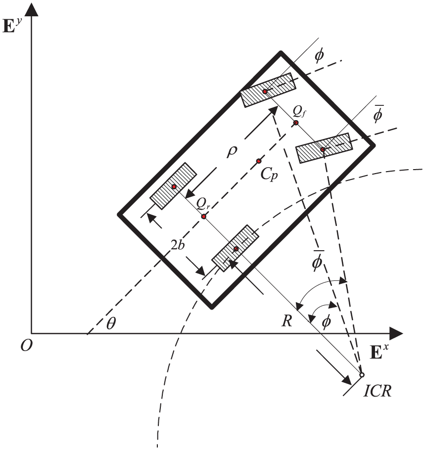
The mobile robot’s turning restrictions.

The relationship between the deviation angle of the left and right wheel can be deduced by the geometrical relationship in the figure

$$\cot \varphi =\frac{R+2b}{\rho },\cot \overline{\varphi }=\frac{R}{\rho }$$

(6)

By the deviation angle drive specification $|\varphi |\le {\varphi }_{max}$ , $|\overline{\varphi }|\le {\overline{\varphi }}_{max}$ , as well as the body geometric parameters, the minimum turning radius when the body turns is determined as

$$R_{min}=\rho \cot {\varphi }_{max}-2b=\rho \cot {\overline{\varphi }}_{max}$$

(7)

$$\frac{1}{\kappa (t)}=\frac{{[{\stackrel{·}{x}}^2(t)+{\stackrel{·}{y}}^2(t)]}^{3/2}}{\stackrel{·}{x}(t)\stackrel{··}{y}(t)-\stackrel{·}{y}(t)\stackrel{··}{x}(t)}$$

(8)

Assuming that the maximum angle of deviation of the actual vehicle is ${\varphi }_{(max)}=25\circ$ , the wheelbase is 1.5 m, and tread is 0.75 m, formula (7) calculates the minimum turning radius of the vehicle body to be about 2.4 m. Basically, the curve obtained by the path planning must be introduced with a limit of curvature called a reasonable motion trajectory. In order for the wheeled robot to be able to successfully turn, the curvature radius $1/\kappa (t)$ of each point on the curve must be greater than the minimum turning radius of the wheeled robot. Given a two-dimensional smoothing curve $S(t)=[x(t),y(t)]$ expressed with time parameter, curvature radius of each point in the curve can be expressed as

$$\frac{1}{\kappa (t)}=\frac{{[{\stackrel{·}{x}}^2(t)+{\stackrel{·}{y}}^2(t)]}^{3/2}}{\stackrel{·}{x}(t)\stackrel{··}{y}(t)-\stackrel{·}{y}(t)\stackrel{··}{x}(t)}$$

(9)

In this way, the minimum turning radius specifications can be used to design the width of the obstacle safety boundary.

• 2. Boundary width design: The design of the safety boundary should not be too wide or too narrow. Too narrow will make collision with obstacles easy and fail to achieve safety protection; too wide will take up too much space to reach the demand of optimization. For example, Figure 5 illustrates how a car’s turning angle at $2\theta$ is used in the design of the obstacle boundary width L.

Figure 5.

Safe boundary width design.

In the figure, $R_{min}$ is the minimum turning radius when the car body turns and the car body length and width are $\ell$ and w, respectively. In addition, $\lambda$ is called the margin (or safety) width, that is, the safe distance for the vehicle body to turn to avoid tripping over obstacles. Herewith, we make $\lambda =\sqrt{{\ell }^2+w^2}/2$ equal to the entire length of the body diagonal.

The safe boundary width design is

$$L_{min}=(\mu +\lambda )\sin \theta =R_{min}(1-\sin \theta )+\lambda \sin \theta$$

(10)

wherein $\mu =(R_{min}/\sin \theta )-R_{min}$

Clearly, to make a car turn smoothly without colliding with an obstacle, boundary width L and turning radius of the vehicle are related to the turning angle.

Convex model of obstacle distribution

This study proposed a modified Dijkstra’s algorithm, combined with the safety boundary concept, to directly use vertices of the convex-shaped obstacle as network nodes. Aimed at the nodes of each obstacle, the cost function assessment was conducted to search for the shortest path. The model information of the obstacles, including the working environment of the robot having m number of convex-shaped obstacles, was obtained by boundary sequence permutation method and turning point detection method. Each obstacle included r_i (i = 1, …, m) number of vertices (or turning points), and its coordinates were expressed as $P_i^j(j=1,2,\dots ,r_i)$ . In order to effectively perform the shortest path search algorithms, the relevant environmental information was re-defined as follows:

• 1. Start point, vertices of each convex-shaped obstacle, and end points in total were

$$k=\sum _{i=1}^m{r}_i+2$$

(11)

To form network nodes, start point coordinates were defined as $D_1(x_1,y_1)$ , vertex coordinates of each obstacle were $D_2(x_2,y_2)~D_{k-1}(x_{k-1},y_{k-1})$ , and end point coordinates were $D_k(x_k,y_k)$ .

The coordinate vector was repressed as follows

$$X=[\begin{array}{cccc}{x}_1\hfill & x_2\hfill & \cdots \hfill & x_k{]}^T\hfill \end{array},Y=[\begin{array}{cccc}{y}_1\hfill & y_2\hfill & \cdots \hfill & y_k{]}^T\hfill \end{array}$$

(12)

• 2. The distance between each network node forms a matrix called the distance matrix, defined as

$$M(i,j)=d_{\mathrm{ij}}=\overline{D_i{D}_j}=\sqrt{{(x_i-x_j)}^2+{(y_i-y_j)}^2}$$

(13)

If obstacles between two network nodes cannot connect with each other, then the corresponding elements in the distance matrix M are defined as $d_{\mathrm{ij}}=\infty$ .

• 3. The cost function from the start point $D_1$ to any network node $D_i$ is defined as $c_i$ , wherein i = 1∼k. The cost function of the start point itself is defined as $c_1=0$ .

• 4. To search in a clockwise direction, all paths including $\widehat{D_1{D}_i},\widehat{D_2{D}_i},\dots ,\widehat{D_{i-1}{D}_i}$ able to reach the D_i node have a total of $i-1$ paths. The cost functions of each path are $c_i^j=c_j+d_{\mathrm{ji}},j=1,2,\dots ,i-1$ , respectively. From these possible paths, a minimum value is selected as the cost function $c_i=min(c_i^1,c_i^2,\dots ,c_i^{i-1})$ from the start point to D_i node. The node tag may be defined as $L(i)=[D_j,c_i=c_j+d_{\mathrm{ji}}]$ , wherein D_j is the so-called source node.

• 5. At the same time, the search path was also defined in a counterclockwise direction. Based on the D_i node for network node $D_p(p=2,\dots ,i-1)$ , all possible paths including $\widehat{D_p{D}_{p+1}},\widehat{D_p{D}_{p+2}},\dots ,\widehat{D_p{D}_i}$ were searched in counterclockwise direction, totaling $i-p$ paths. The cost function of counterclockwise search mode was expressed as $c^{*}$ .

The forbidden path judgment

It is assumed that the mobile robot moves in the $R^2$ plane and all obstacles are of convex collection. Figure 9 illustrates the so-called forbidden path. Consider the distance between nodes $D_1=(x_1,y_1)$ and $D_5=(x_5,y_5)$ . According to formula (13), the calculation should be $\sqrt{{(x_1-x_5)}^2+{(y_1-y_5)}^2}$ , but as obstacle ${\mathrm{\Omega }}_1$ exists between two nodes, connection is impossible. The elements in the distance matrix should be modified to $M(1,5)=\infty$ . In order to effectively achieve this, this study proposed the judgment method of the forbidden path to decide whether or not the two nodes are connected. The most important task is to establish a complete obstacle model. First, we start from the definition of a collection of a straight line

$$L=\left\{D|{\alpha }^T(D-D_0)=0\right\}$$

(14)

wherein $\alpha \in R^2$ is the perpendicular vector of this line, $D_0=(x_0,y_0{)}^T\in R^2$ is any point on this line, and $D=(x,y{)}^T\in R^2$ . Therefore, $D-D_0$ and $\alpha$ are the two orthogonal vectors. The straight line represented by formula (14) can divide the $R^2$ plane into two parts, as shown in Figure 6. ${\alpha }^{T}D\ge \beta$ represents a half-plane (e.g. shaded) in the same direction with $\alpha$ vector, and ${\alpha }^{T}D\le \beta$ represents the half-plane in the opposite direction with $\alpha$ vector. The polygonal obstacle $\mathrm{\Omega }$ in this study can be described by the above method, as shown in Figure 7. The obstacle is composed of r number of half-planes, and the normal vectors ${\alpha }_1,{\alpha }_2,\dots ,{\alpha }_r$ of each linear equation L are outwardly defined. The obstacle model can be expressed as follows

$$\mathrm{\Omega }=\{\mathrm{\Delta }|({\alpha }_1^{T}D\le {\beta }_1)\cap ({\alpha }_2^{T}D\le {\beta }_2)\cap \cdots \cap ({\alpha }_r^{T}D\le {\beta }_r)\}$$

(15)

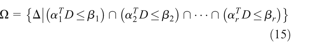
wherein “∩” stands for the significance of “and.”

Figure 6.

Indication of linear equation cutting plane.

Figure 7.

Indication of polygon obstacle model.

The use of the polygon obstacle model (Figure 7) is conducive to the resolution of the problem whether or not the forbidden path lies between two nodes. The judgment criterion and the relevant steps are stated as follows:

• Step 1: Via the turning point detection, the vertex coordinates of each obstacle were found to be $P_i^j(j=1,2,\dots ,r_i)$ .

• Step 2: For the two turning points of each obstacle (called vertices), a linear equation was determined. For example, in the ith obstacle, formula (14) using $\overline{P_i^1{P}_i^2},\overline{P_i^2{P}_i^3},\dots ,\overline{P_i^{r_i}{P}_i^1}$ , respectively, determined $L_i^1,L_i^2,\dots ,L_i^{r_i}$ number of equations. Furthermore, formula (15) obtained the geometric model ${\mathrm{\Omega }}_i$ of the obstacle, wherein $i=1,2,\dots ,m$ .

• Step 3: Regarding the start point, vertices of all obstacles, and end points in the image as network nodes $D_1~D_k$ , using the vector of the coordinates of each point, the distance and slope between all network nodes are easily calculated. However, the judgment of the forbidden path confirmed whether or not the two nodes connected, that is, whether or not there was an obstacle between two nodes.

• Step 4: Any two nodes $D_a$ and $D_b$ were taken for illustration, so as to determine whether the two nodes connected. From the initial node $D_a$ to the destination node $D_b$ , the corresponding x coordinate is increased by 1 in sequence, that is, from $x_a+1$ to $x_b-1$ . Through the slope obtained in Step 3, all corresponding y coordinates were found and these points were called detection points, as shown in Figure 8. $D_t=(x_t,y_t{)}^T$ was assumed to be a detection point; when it simultaneously satisfied the following $r_i$ number of conditions

  $$\begin{array}{l}\left({\alpha }_i^1{D}_t\le {\beta }_i^1\right)\cap \left({\alpha }_i^2{D}_t\le {\beta }_i^2\right)\cap \mathrm{\dots }\cap \left({\alpha }_i^{r_i}{D}_t\le {\beta }_i^{r_i}\right),\\ i=1,2,\mathrm{\dots },m\end{array}$$

  then it was called the detection point $D_t$ , which fell in the range covered by the polygonal obstacle ${\mathrm{\Omega }}_i$ . Then, the two nodes $D_a$ and $D_b$ were not connected, and the distance matrix was $M(a,b)=\infty$ .

Figure 8.

Using detection point for discrimination of forbidden path.

Modified Dijkstra’s algorithm

Consider k number of network nodes $D_1~D_k$ during evaluation of the cost function of a node. This article applied two-way search skills to propose a modified Dijkstra’s algorithm, divided into two modes of clockwise search and counterclockwise search. First, the cost function of the start point D₁ was set as 0, namely, $c_1=0$ . Followed by calculation of the cost function of D₂ node, a search was conducted in the forward mode. Its only path was $\widehat{D_1{D}_2}$ , so the forward mode cost function was $c_2=c_1+d_{12}$ , and the node tag was defined as $L(2)=[D_1,c_2=c_1+d_{12}]$ . Following consideration of D₃ nodes, the two paths $\widehat{D_1{D}_3}$ and $\widehat{D_2{D}_3}$ were compared to determine node tag $L(3)$ with cost function of shortest path. Each node $D_i(i=2~k)$ in the forward mode was sequentially evaluated, and the node was marked and defined as $L(i)=[D_u,c_i=c_u+d_{\mathrm{ui}}]$ , wherein $D_u$ indicates the source node of $D_i$ . To evaluate the cost function in the forward mode, consider only the path of a smaller mark, D_i node. For example, consider only the path $\widehat{D_j{D}_i}(j=1,2,\dots ,i-1)$ . In the forward search process, once the cost function of D_i node is found to be much smaller than last node D_i−1, it means a shorter path may appear in the start reverse search from D_i. In this case, the algorithm will be changed to reverse search, the cost function of all previous nodes must be re-evaluated in counterclockwise direction, and compared to the result of the forward search, the shortest path to reach the target of total field search is re-determined. For example, in the reverse search mode of D_p nodes, all possible paths including $\widehat{D_p{D}_{p+1}}(q=p+1~i)$ leading to the D_p node are evaluated with the minimum cost function to get $c_p^{*}=c_v+d_{\mathrm{vp}}$ , which indicates that $D_v$ is the source node of $D_p$ reverse search. After path searching through the two modes, comparison at the end showed the forward mode or reverse mode can achieve optimal path planning. The event $c_p<c_p^{*}$ means the forward mode can find a path with a smaller cost function, and the D_p node tag remains unchanged. The event $c_p>c_p^{*}$ means the effect of reverse search is better than the original, and the original node tag must be corrected as $L(p)=[D_v,c_p=c_v+d_{\mathrm{vp}}]$ . The cost function of each node was calculated according to the above process, and a complete forward and reverse search evaluation was conducted in order to update the network tag of all nodes. Finally, from the node tag of end point D_k, the source node was searched for in order until start point D₁. Connecting D₁, the relay node, and D_k constitutes the so-called shortest path.

After execution, c is smallest element value in the x-vector; I is the indicator value of the smallest element located in the x-vector.

Figure 9 shows two obstacles, ${\mathrm{\Omega }}_1$ and ${\mathrm{\Omega }}_2$ , respectively. After the turning point detection image processing, all network vertex coordinates were $D_1=(0,0)$ , $D_2=(5,5)$ , $D_3=(3,9)$ , $D_4=(5,13)$ , $D_5=(10,13)$ , $D_6=(12,9)$ , $D_7=(10,5)$ , $D_8=(14,15)$ , $D_9=(13,16)$ , $D_{10}=(17,23)$ , $D_{11}=(19,23)$ , $D_{12}=(23,16)$ , $D_{13}=(22,15)$ , and $D_{14}=(25,25)$ . This study proposed a modified Dijkstra’s algorithm to search for the shortest path from start point $D_1$ to end point $D_{14}$ . The table on the right shows the hand count process for each network node. Worth noting are nodes $D_6$ and $D_{12}$ . A reverse search found that when source nodes were $D_7$ and $D_{13}$ , it obtained the cost function with the shortest path. Of course, this is due to the cost functions $c_7<c_6$ and $c_{13}<c_{12}$ . The node tag of end point $D_{14}$ was found from its source node $D_{12}$ , and search forward in sequence until initial node $D_1$ was then conducted from node tag $D_{12}$ . The shortest path was found to be $D_1\to D_7\to D_{13}\to D_{12}\to D_{14}$ .

Figure 9.

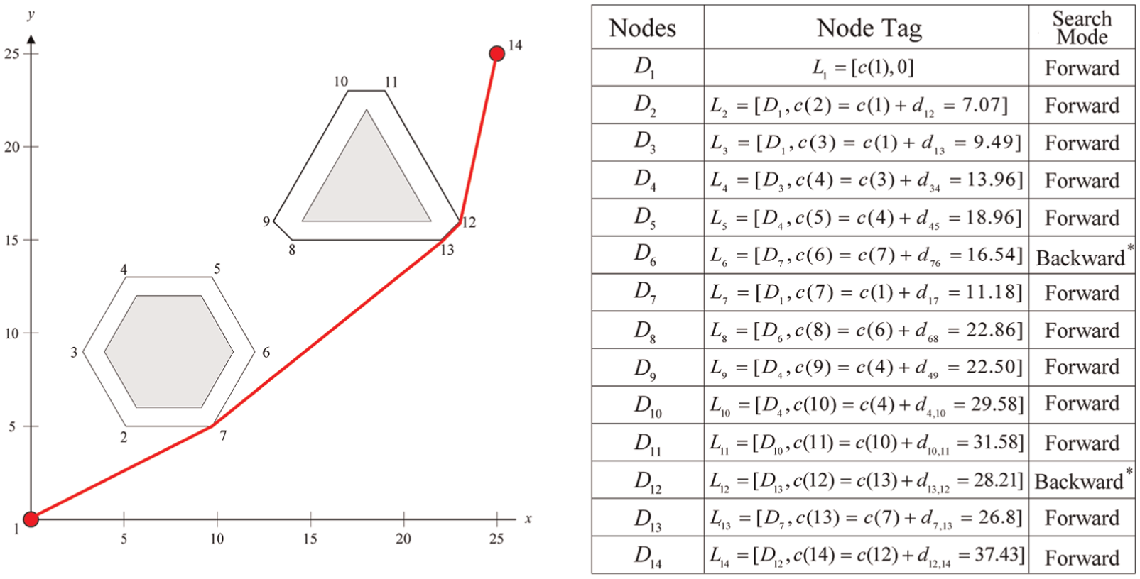
Modified Dijkstra’s algorithm hand count process.

Simulation results

Case 1

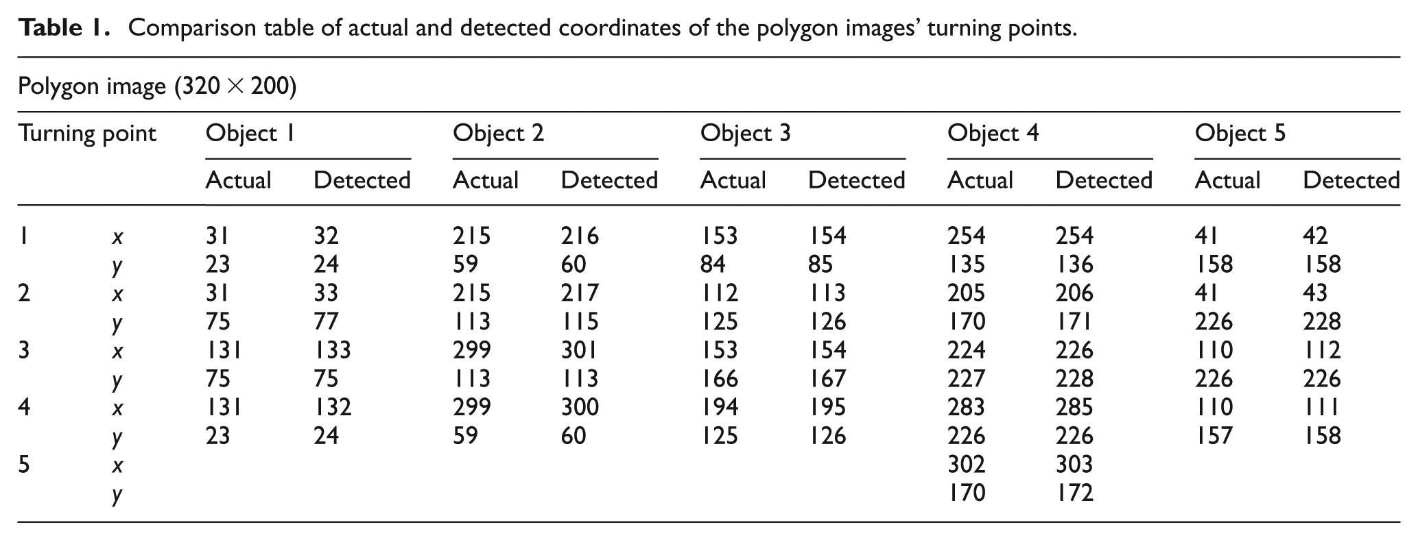
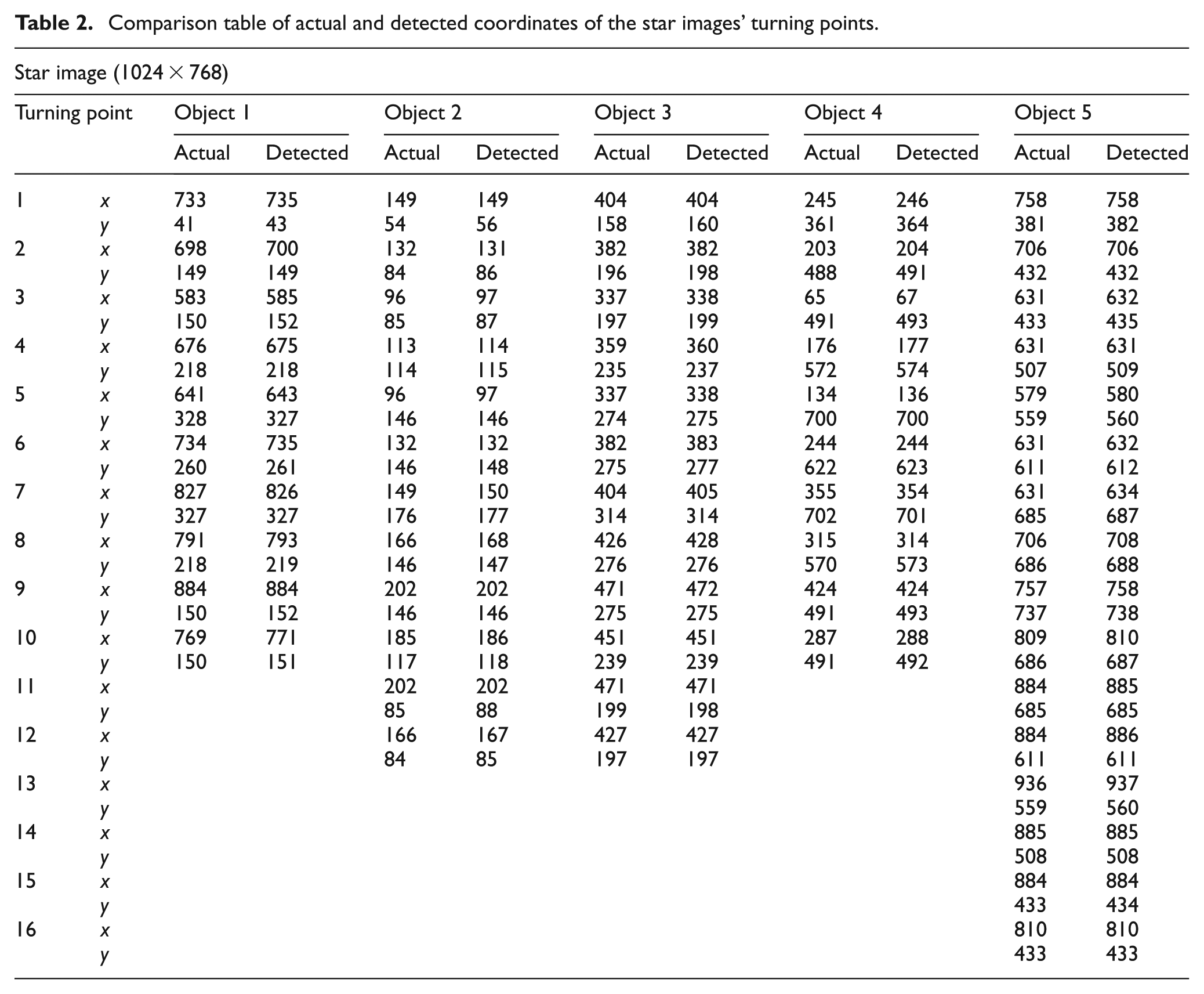
Using the programming language MATLAB 7.0, the proposed boundary sequence permutation of this study and the turning point detection algorithm were used to conduct simulation validation; Figures 10 and 11 illustrate the processing results of the turning point detection method, and Tables 1 and 2 record the comparison of the turning point actual coordinates and the actual detection results of the algorithms. First, the boundary sequence permutation of objects was used to complete the recording of the number of objects in the image and the edge point permutation coordinates of each object. Then, the turning point detection algorithm was used to identify the point of curvature value greater than threshold value, $T_c$ . This point is likely the turning point that we want to detect. Finally, through the selection of the neighbor radius r to filter the pseudo turning point, the maximum curvature value from the adjacent interval was found in order to determine the real turning point. The turning point detected in the figure was depicted with a circle on the edge of the object for easy identification. In addition, the digital images generated digitizing errors, so we inevitably had 0∼3 pixel errors in the detection process; refer to Tables 1 and 2. The experimental results suggest that the method proposed in this study not only has a good effect of turning point detection but also has a high practical value.

Figure 10.

Polygon images.

Figure 11.

Star images.

Table 1.

Comparison table of actual and detected coordinates of the polygon images’ turning points.

Polygon image (320 × 200)
Turning point		Object 1		Object 2		Object 3		Object 4		Object 5
		Actual	Detected	Actual	Detected	Actual	Detected	Actual	Detected	Actual	Detected
1	x	31	32	215	216	153	154	254	254	41	42
	y	23	24	59	60	84	85	135	136	158	158
2	x	31	33	215	217	112	113	205	206	41	43
	y	75	77	113	115	125	126	170	171	226	228
3	x	131	133	299	301	153	154	224	226	110	112
	y	75	75	113	113	166	167	227	228	226	226
4	x	131	132	299	300	194	195	283	285	110	111
	y	23	24	59	60	125	126	226	226	157	158
5	x							302	303
	y							170	172

Table 2.

Comparison table of actual and detected coordinates of the star images’ turning points.

Star image (1024 × 768)
Turning point		Object 1		Object 2		Object 3		Object 4		Object 5
		Actual	Detected	Actual	Detected	Actual	Detected	Actual	Detected	Actual	Detected
1	x	733	735	149	149	404	404	245	246	758	758
	y	41	43	54	56	158	160	361	364	381	382
2	x	698	700	132	131	382	382	203	204	706	706
	y	149	149	84	86	196	198	488	491	432	432
3	x	583	585	96	97	337	338	65	67	631	632
	y	150	152	85	87	197	199	491	493	433	435
4	x	676	675	113	114	359	360	176	177	631	631
	y	218	218	114	115	235	237	572	574	507	509
5	x	641	643	96	97	337	338	134	136	579	580
	y	328	327	146	146	274	275	700	700	559	560
6	x	734	735	132	132	382	383	244	244	631	632
	y	260	261	146	148	275	277	622	623	611	612
7	x	827	826	149	150	404	405	355	354	631	634
	y	327	327	176	177	314	314	702	701	685	687
8	x	791	793	166	168	426	428	315	314	706	708
	y	218	219	146	147	276	276	570	573	686	688
9	x	884	884	202	202	471	472	424	424	757	758
	y	150	152	146	146	275	275	491	493	737	738
10	x	769	771	185	186	451	451	287	288	809	810
	y	150	151	117	118	239	239	491	492	686	687
11	x			202	202	471	471			884	885
	y			85	88	199	198			685	685
12	x			166	167	427	427			884	886
	y			84	85	197	197			611	611
13	x									936	937
	y									559	560
14	x									885	885
	y									508	508
15	x									884	884
	y									433	434
16	x									810	810
	y									433	433

Case 2

The MATLAB graphical user interface (GUI) toolbox was used to write the simulation software for obstacle avoidance paths, performed under a 2.8-GHz Pentium 4 processor. This study proposed the combination of boundary sequence permutation method, turning point detection method, forbidden path detection method, and modified Dijkstra’s shortest path search in a multi-functional integrated window. The image captured by the CCD or the users’ own selection set the obstacle distribution in the environment model. For example, the working interval in Figure 12(a) shows the coordinates of the starting point to be (0, 0) and the end point coordinates (25, 25). The user selected a triangular obstacle with a central point at (10, 5) and a radius of 3, a pentagonal obstacle with a central point at (15, 15) and a radius of 3, and a hexagonal obstacle with a central point at (20, 20) and a radius of 2. The goal was to design the shortest path curve from the start point to the end point coordinates. The turning point detection algorithm of image processing obtained a total of $D_1~D_{19}$ number of network nodes. By the path planning button, the modified Dijkstra’s algorithm derived the shortest path $D_1\to D_9\to D_{15}\to D_{19}$ , as shown in Figure 12(b). Figure 13(a) slightly moved the pentagonal obstacle to the left, making the center point at (12, 15). Interestingly, the path planning result turned out to be very different. The shortest path became $D_1\to D_4\to D_{12}\to D_{11}\to D_{14}\to D_{15}\to D_{19}$ , as shown in Figure 13(b).

Figure 12.

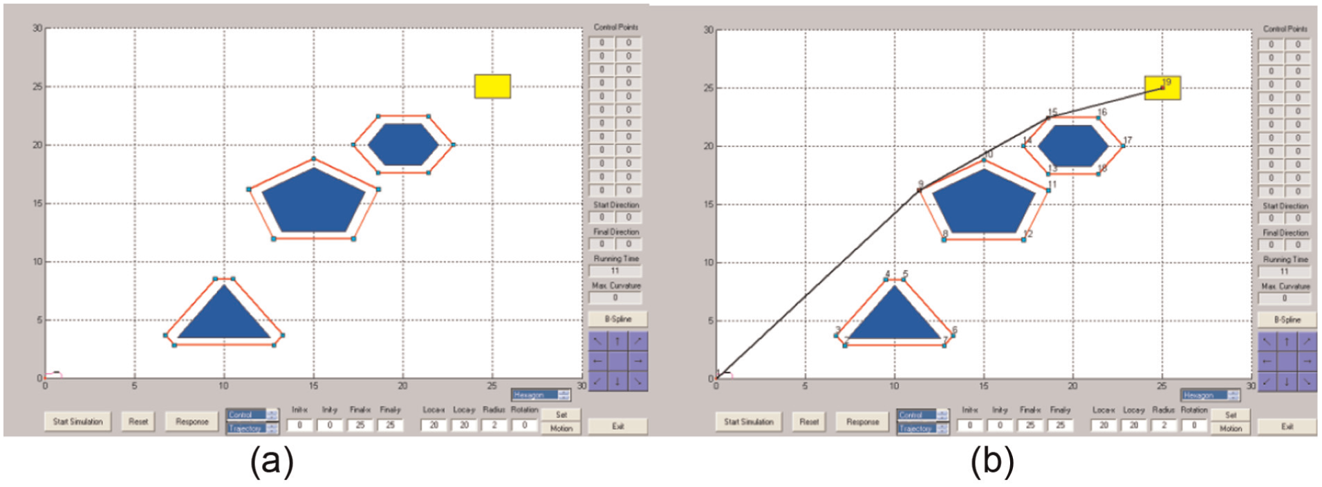
(a) Obstacle distribution and (b) path planning results.

Figure 13.

(a) Obstacle distribution and (b) path planning results.

Conclusion

The main purpose of this study is to identify and avoid obstacles using images to plan out the shortest and smoothest obstacle-avoiding path. Through the boundary sequence permutation method and Rosenfeld–Johnston’s turning point detection algorithm, all the turning point coordinates of the object were measured. The modified Dijkstra’s algorithm was used to find an obstacle-avoiding path connecting the start point, turning point of the obstacle, and end point. Compared with the traditional method, the method proposed achieved the goals of global search by forward and reverse modes. To direct future improvements, the discovery of digitizing errors through the simulation process is an important factor affecting detection results.