Coupled analysis of two-dimensional acoustic and membrane vibration by concentrated mass model: Proposal of spurious mode elimination model

Abstract

When using the finite element method for structural–acoustic coupled analysis, the mass and stiffness matrices are not symmetric because the acoustic space is described by sound pressure and the structure is described by displacement. Therefore, eigenvalue analysis requires a long computational time. In this article, we proposed concentrated mass models for performing structural–acoustic coupled analysis. The advantage of this model is that the mass and stiffness matrices become symmetric because both the acoustic space and the membrane are described by the displacement of the mass points. Furthermore, our models do not generate spurious modes and zero eigenvalues that arise in finite element method whose variable is displacement in acoustic space. To validate the proposed models, the natural frequency obtained using the concentrated mass models is compared with the natural frequency found using finite element method. These results are in good agreement, and spurious modes and zero eigenvalues are not generated in the proposed model whose variables are sound pressure. Furthermore, we compare the proposed model with finite element method in terms of the calculation time required for the eigenvalue analysis. Because the matrices of the proposed models are symmetric, these eigenvalue analyses are faster than that of finite element method, whose matrices are asymmetric. Therefore, we conclude that the proposed model is valid for coupled analysis of a two-dimensional acoustic space and membrane vibration and that it is superior to finite element method in terms of calculation time.

Introduction

To reduce interior noise in transportation vehicles, structural–acoustic coupled analyses have been performed using the finite element method (FEM).^1–3 Craggs ⁴ and Everstine et al. ⁵ gave equations of motion in FEM for the structural–acoustic coupled problem. However, the derivation of these equations is complicated because of the different variables in the structural and acoustic fields. In the structural field, displacement at the nodal point is used as the variable, whereas in the acoustic field, sound pressure or velocity potential is used. Therefore, the mass and stiffness matrices of the equation of motion are asymmetric. This asymmetry increases the computational time required for eigenvalue analysis of the coupled problem and complicates modal analysis because orthogonality is not satisfied. ⁶

To overcome the problem of eigenvalue analysis, Craggs and Stead ⁷ arranged frequency domain equations into a symmetric form. However, this method cannot be applied to damped systems.

To overcome the problems of eigenvalue and modal analysis, many researchers have transformed asymmetric equations of motion into symmetric equations. Everstine ⁸ substituted the coupled term into the damping matrix to symmetrize the mass and stiffness matrices. Olson and Bathe ⁹ introduced air velocity potential in addition to sound pressure and derived a symmetric equation with a damping matrix. However, such approaches require solving complex eigenvalue problems, even in the case of an undamped system or proportional viscous damping. Ohayon^10,11 and Sandberg and Goransson ¹² introduced air displacement potential as a replacement for velocity potential and derived a symmetric equation that does not have a damping matrix. However, the degree of freedom is redundant, and the mass and stiffness matrices are dense, thus requiring a long computational time. MacNeal et al.^13,14 and Sandberg ¹⁵ transformed sound pressure in the acoustic field and displacement in the structure into modal coordinates and arranged the equation of motion as a symmetric equation using coordinate transformation. Flanigan and Borders ¹⁶ analyzed acoustic and panel vibration problems using MacNeal’s method. However, these approaches require that eigenvalue analysis of the acoustic field and structure be done in advance. Moreover, as a result of the coordinate transformation, the physical meaning of the original coordinates is lost, despite its importance in system-parameter identification problems. ⁶

To overcome the problem of modal analysis when an asymmetric equation is used, Hagiwara and Ma ¹⁷ introduced the concept of left and right eigenvectors to perform modal analysis using asymmetric equations of motion. However, the eigenvalue problem is asymmetric in the first modal analysis step, and so considerable computational time is required for eigenvalue analysis.

The other methods to overcome these problems are FEMs whose variable is displacement in the acoustic space.^18–20 These methods have the advantage that the compatibility and equilibrium condition along the boundary between the acoustic space and the structure is satisfied easily, ²⁰ and the mass and stiffness matrices are symmetric. However, zero eigenvalues whose natural frequencies are 0 Hz and spurious modes that are physically meaningless are generated in these methods.^18,20 Hori et al. ²¹ and Kim and Yun ²⁰ proposed the methods to transform the spurious modes into zero eigenvalues. However, the degree of freedom is larger than that of FEM with sound pressure or velocity potential as the variable.

In our previous study, we proposed a concentrated mass model for coupled analysis of two-dimensional acoustic and membrane vibration. ²² This model consists of masses and connecting springs. The mass points are placed at the intersection points of elements, and the displacement of the mass point is used as the variable in this model. For the structural–acoustic coupled problem, the treatment of the coupling involves only placing the mass points of the structure and of the acoustic field at the nodal points in each area. Therefore, the equations of motion of the mass points can be derived simply. Furthermore, the mass and stiffness matrices in the equations are symmetric. Thus, the modal analysis can be applied easily, and the computational cost of the eigenvalue analysis becomes lower when using the concentrated mass model. However, zero eigenvalues and spurious modes are also generated in this model. ²²

Here, we propose a new concentrated mass model to eliminate the zero eigenvalues and spurious modes. The sound space and membrane are modeled as masses and connecting springs. The mass points are placed at the center of sides of elements to eliminate the spurious modes. Furthermore, the variable displacements of the mass points are transformed into the sound pressure to eliminate zero eigenvalues. To validate the proposed model, the natural frequency obtained by the concentrated mass model is compared with that obtained by FEM.

Concentrated mass model

We deal with a coupled problem of a two-dimensional acoustic in a rectangular plate-shaped space and one-dimensional membrane vibration, as shown in Figure 1. One face of the rectangular plate-shaped space is the membrane and the other faces are rigid. The thickness of the acoustic space is h. The lengths of the acoustic space are $L_x$ and $L_y$ in the x and y directions. The air in the acoustic space and the membrane are modeled as a concentrated mass model that consists of masses and connecting springs.

Figure 1.

Analytical space.

Model of acoustic space

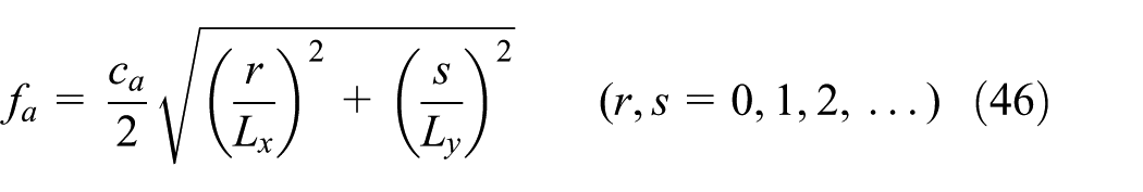
The air in the acoustic space is modeled as a concentrated mass that consists of masses and connecting springs, as shown in Figure 2. The space is divided into uniform rectangular elements with sides of $l_x$ and $l_y$ (Figure 3). The division numbers are $N_x$ and $N_y$ in the x and y directions. The mass is concentrated at the center of each side. The masses located on both the right and the left sides have displacement in the x direction, $x_{i,j}$ , and those located on both the top and the bottom sides have displacement in the y direction, $y_{i,j}$ . The sound pressure in element $[i,j]$ is $d{p}_{i,j}$ . The pressure in the equilibrium state is $p_0$ , density in the equilibrium state is ${\rho }_0$ , and volume in each element in the equilibrium state is $V_0=h{l}_x{l}_y$ . Considering the mass of air in the shaded area in Figure 4, the mass of each mass point is

$$m_a={\rho }_{0}h{l}_x{l}_y$$

(1)

A connecting spring describes the relationship between pressure $d{p}_{i,j}$ and volume $V_{i,j}$ in each element. If we treat the fluid as an ideal gas and assume an adiabatic change, we obtain

$$p_0{V}_0^{\gamma }=(p_0+d{p}_{i,j})(V_0+d{V}_{i,j}{)}^{\gamma }$$

(2)

where $\gamma$ is the ratio of specific heats, and $d{V}_{i,j}$ is the variation of volume in element [i, j]. If we assume that the element volume changes, as shown in Figure 5 when the mass points move,

$d{V}_{i,j}$ is given by

$$d{V}_{i,j}=h\{l_y(x_{i,j}-x_{i-1,j})+l_x(y_{i,j}-y_{i,j-1})\}$$

(3)

Substituting equation (3) into equation (2) and linearizing, we obtain

$$d{p}_{i,j}=-\frac{p_0\gamma h}{V_0}\{l_y(x_{i,j}-x_{i-1,j})+l_x(y_{i,j}-y_{i,j-1})\}$$

(4)

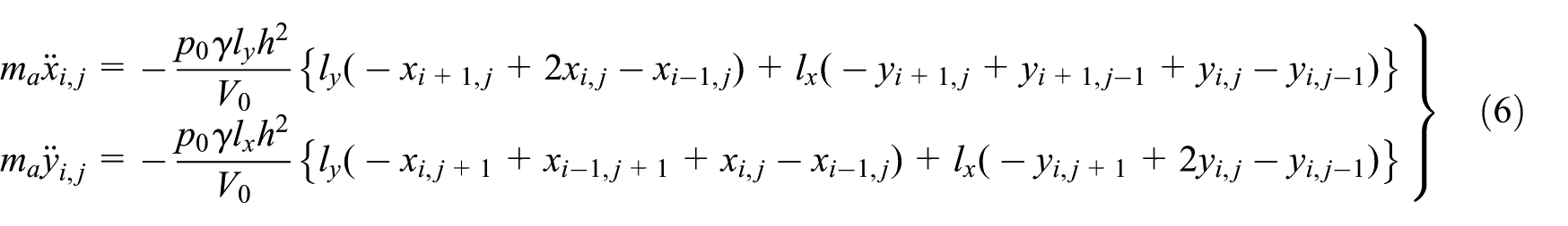
Considering the force acting on the shaded area in Figure 4, the equations of motion in the x and y directions are given by

$$\begin{array}{c}{m}_a{\stackrel{··}{x}}_{i,j}=l_{y}h(d{p}_{i,j}-d{p}_{i+1,j})\hfill \\ \multicolumn{1}{c}{m_a{\stackrel{··}{y}}_{i,j}=l_{x}h(d{p}_{i,j}-d{p}_{i,j+1})}\end{array}\}$$

(5)

Substituting equation (4) into equation (5), the equations of motion can be written as follows using the displacements

$$\begin{array}{c}{m}_a{\stackrel{··}{x}}_{i,j}=-\frac{p_0\gamma l_y{h}^2}{V_0}\{l_y(-x_{i+1,j}+2x_{i,j}-x_{i-1,j})+l_x(-y_{i+1,j}+y_{i+1,j-1}+y_{i,j}-y_{i,j-1})\}\hfill \\ \multicolumn{1}{c}{m_a{\stackrel{··}{y}}_{i,j}=-\frac{p_0\gamma l_x{h}^2}{V_0}\{l_y(-x_{i,j+1}+x_{i-1,j+1}+x_{i,j}-x_{i-1,j})+l_x(-y_{i,j+1}+2y_{i,j}-y_{i,j-1})\}}\end{array}\}$$

(6)

Figure 2.

Concentrated mass model.

Figure 3.

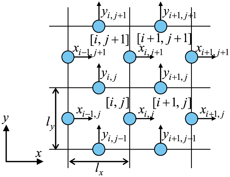
Square lattice and mass point.

Figure 4.

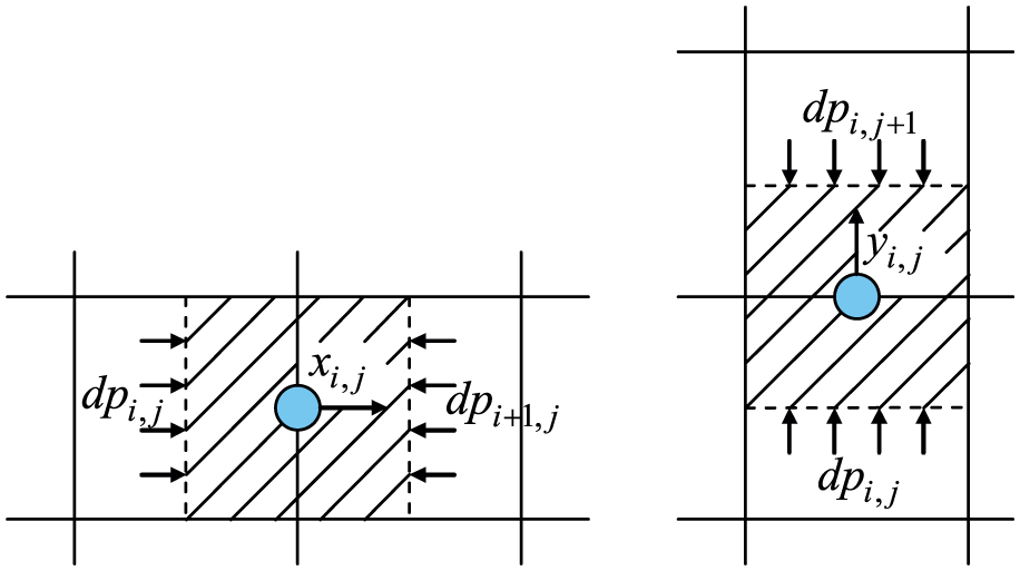
Definition of mass and sound pressure force.

Figure 5.

Volume variation in element $[i,j]$ .

Membrane model

The membrane face in Figure 1 is modeled as a concentrated mass model that consists of masses and connecting springs, as shown in Figure 6. We consider a one-dimensional membrane. The membrane is divided into uniform elements such that the length is $l_y$ (Figure 7) and the number of divisions is $N_y$ . The mass is concentrated at the nodal point. The displacement of the nodal point j in the x-direction is ${\xi }_j$ , the membrane tension is $T_m$ , and the surface density is ${\rho }_m$ .

Figure 6.

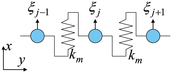
Membrane model.

Figure 7.

Membrane element.

Considering the mass of the membrane in the shaded area in Figure 7, the mass of each mass point is

$$m_m={\rho }_{m}h{l}_y$$

(7)

The restoring force of the membrane is modeled as a spring. The forces shown in Figure 8 act on the shaded area shown in Figure 7. The displacement of the membrane at coordinate y in the x-direction is $\xi (y)$ . The x-direction component of the tension from the left side is $T_m(\partial \xi /\partial y{)}_L$ , and therefore, the restoring force from the left side becomes

$$f_m=T_{m}h{\left(\frac{\partial \xi }{\partial y}\right)}_L$$

(8)

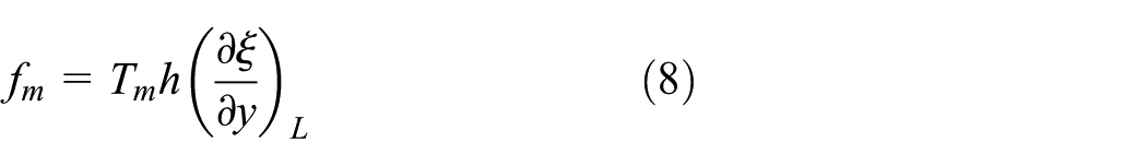
If we relate $\xi$ to the displacement of the mass point ${\xi }_j$ and transform equation (8) to the finite difference form, we get

$$f_m=T_{m}h\frac{{\xi }_j-{\xi }_{j-1}}{l_y}$$

(9)

From this equation, the constant of the spring shown in Figure 6 is

$$k_m=\frac{T_{m}h}{l_y}$$

(10)

Figure 8.

Tension of membrane.

Treatment of coupled region

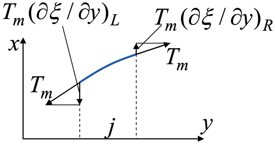
Next, we treat the coupled region of the acoustic space and the membrane. Figure 9 shows the mass arrangement in the $x-y$ plane in the vicinity of the membrane. The heavy line on the right side indicates the membrane, and the left-hand side of the membrane is acoustic space. Considering the variation in the volume next to the membrane using the displacements of the mass points of the membrane and acoustic space, the sound pressure in element [ $N_x$ , j] is given by

$$d{p}_{N_x,j}=-\frac{p_0\gamma h}{V_0}\{l_y({\xi }_j-x_{N_x-1,j})+l_x(y_{N_x,j}-y_{N_x,j-1})\}$$

(11)

Figure 9.

Placement of mass point near membrane.

Assuming that the mass of the mass point on the membrane is the sum of the membrane mass and the air mass in half of the element and that the sound pressure, $d{p}_{N_x,j}$ , acts on mass point j of the membrane, the equation of motion of the membrane mass point becomes

$$(m_m+\frac{m_a}{2}){\stackrel{··}{\xi }}_j=k_m({\xi }_{j+1}-2{\xi }_j+{\xi }_{j-1})+l_y\mathrm{hd}{p}_{N_x,j}$$

(12)

Substituting equation (11) into equation (12), the equation of motion is given as follows using the displacement of the mass points of air

$$\begin{array}{c}(m_m+\frac{m_a}{2}){\stackrel{··}{\xi }}_j=k_m({\xi }_{j+1}-2{\xi }_j+{\xi }_{j-1})\hfill \\ -\frac{p_0\gamma l_y{h}^2}{V_0}\{l_y({\xi }_j-x_{N_x-1,j})+l_x(y_{N_x,j}-x_{N_x,j-1})\}\hfill \end{array}$$

(13)

Equation of motion

Arranging equations (6) and (13) in a matrix gives equations in the form

$$\left[\begin{array}{cc}{\mathbf{M}}_{\mathrm{aa}}\hfill & 0\hfill \\ \multicolumn{1}{c}{0}& {\mathbf{M}}_{\mathrm{mm}}\hfill \end{array}\right]\left[\begin{array}{c}\stackrel{··}{\mathbf{x}}\hfill \\ \multicolumn{1}{c}{\stackrel{··}{\mathbf{\xi }}}\end{array}\right]+\left[\begin{array}{cc}{\mathbf{K}}_{\mathrm{aa}}\hfill & {\mathbf{K}}_{\mathrm{am}}\hfill \\ \multicolumn{1}{c}{{\mathbf{K}}_{\mathrm{ma}}}& {\mathbf{K}}_{\mathrm{mm}}\hfill \end{array}\right]\left[\begin{array}{c}\mathbf{x}\hfill \\ \multicolumn{1}{c}{\mathbf{\xi }}\end{array}\right]=\left[\begin{array}{c}0\hfill \\ \multicolumn{1}{c}{0}\end{array}\right]$$

(14)

where $\mathbf{x}$ is the displacement vector whose elements are the displacements $x_{i,j},y_{i,j}$ in the acoustic space; $\mathbf{\xi }$ is the displacement vector whose elements are the displacement ${\xi }_j$ of the membrane; ${\mathbf{M}}_{\mathrm{aa}}$ and ${\mathbf{M}}_{\mathrm{mm}}$ are mass matrices whose on-diagonal elements are the masses of the acoustic space and membrane, respectively; ${\mathbf{K}}_{\mathrm{aa}}$ and ${\mathbf{K}}_{\mathrm{mm}}$ are the stiffness matrices of the acoustic space and membrane, respectively; and ${\mathbf{K}}_{\mathrm{am}}$ and ${\mathbf{K}}_{\mathrm{ma}}$ are the stiffness matrices in the coupled region. The matrices in equation (14) are symmetric because ${\mathbf{M}}_{\mathrm{aa}}$ , ${\mathbf{M}}_{\mathrm{mm}}$ , ${\mathbf{K}}_{\mathrm{aa}}$ , and ${\mathbf{K}}_{\mathrm{mm}}$ are symmetric and ${\mathbf{K}}_{\mathrm{am}}={\mathbf{K}}_{\mathrm{ma}}^T$ , so the computational time for eigenvalue analysis becomes small.

Sound pressure model

The degree of freedom of equation (14) is redundant because the variables in the acoustic space are $x_{i,j},y_{i,j}$ , the number of which is twice that of sound pressure $d{p}_{i,j}$ . Therefore, zero eigenvalues whose natural frequencies are 0 Hz are generated when the eigenvalue problem of equation (14) is solved. To reduce the degree of freedom of the acoustic space, the displacements $x_{i,j},y_{i,j}$ are transformed into the sound pressure $d{p}_{i,j}$ .

Arranging equations (4) and (11) in a matrix gives equations in the form

$$\mathbf{p}={\mathbf{T}}_{\mathrm{aa}}\mathbf{x}+{\mathbf{T}}_{\mathrm{am}}\mathbf{\xi }$$

(15)

where $\mathbf{p}$ is the vector whose elements are sound pressure $d{p}_{i,j}$ , and ${\mathbf{T}}_{\mathrm{aa}}$ and ${\mathbf{T}}_{\mathrm{am}}$ are transformation matrices. Arranging equations (5) and (12) in a matrix gives the following equation using $\mathbf{p}$

$$\left[\begin{array}{cc}{\mathbf{M}}_{\mathrm{aa}}\hfill & 0\hfill \\ \multicolumn{1}{c}{0}& {\mathbf{M}}_{\mathrm{mm}}\hfill \end{array}\right]\left[\begin{array}{c}\stackrel{··}{\mathbf{x}}\hfill \\ \multicolumn{1}{c}{\stackrel{··}{\mathbf{\xi }}}\end{array}\right]+\left[\begin{array}{cc}{\overline{\mathbf{K}}}_{\mathrm{aa}}\hfill & 0\hfill \\ \multicolumn{1}{c}{{\overline{\mathbf{K}}}_{\mathrm{ma}}}& {\mathbf{K}}_{\mathrm{mm}}\hfill \end{array}\right]\left[\begin{array}{c}\mathbf{p}\hfill \\ \multicolumn{1}{c}{\mathbf{\xi }}\end{array}\right]=\left[\begin{array}{c}0\hfill \\ \multicolumn{1}{c}{0}\end{array}\right]$$

(16)

where ${\overline{\mathbf{K}}}_{\mathrm{aa}}$ and ${\overline{\mathbf{K}}}_{\mathrm{ma}}$ are the stiffness matrices when sound pressure is used. The relationship between ${\mathbf{T}}_{\mathrm{aa}}$ and ${\overline{\mathbf{K}}}_{\mathrm{aa}}$ and that between ${\mathbf{T}}_{\mathrm{am}}$ and ${\overline{\mathbf{K}}}_{\mathrm{ma}}$ becomes

$$\begin{array}{c}{\overline{\mathbf{K}}}_{\mathrm{aa}}=\alpha {\mathbf{T}}_{\mathrm{aa}}^T\hfill \\ \multicolumn{1}{c}{{\overline{\mathbf{K}}}_{\mathrm{ma}}=\alpha {\mathbf{T}}_{\mathrm{am}}^T}\end{array}\}$$

(17)

where $\alpha =V_0/p_0\gamma$ . Substituting equation (17) into equation (16), the equation of motion becomes

$$\left[\begin{array}{cc}{\mathbf{M}}_{\mathrm{aa}}\hfill & 0\hfill \\ \multicolumn{1}{c}{0}& {\mathbf{M}}_{\mathrm{mm}}\hfill \end{array}\right]\left[\begin{array}{c}\stackrel{··}{\mathbf{x}}\hfill \\ \multicolumn{1}{c}{\stackrel{··}{\mathbf{\xi }}}\end{array}\right]=\left[\begin{array}{cc}{\mathbf{T}}_{\mathrm{aa}}^T\hfill & 0\hfill \\ \multicolumn{1}{c}{{\mathbf{T}}_{\mathrm{am}}^T}& \mathbf{I}\hfill \end{array}\right]\left[\begin{array}{c}-\alpha \mathbf{p}\hfill \\ \multicolumn{1}{c}{-{\mathbf{K}}_{\mathrm{mm}}\mathbf{\xi }}\end{array}\right]$$

(18)

Here, $\mathbf{I}$ is a unit matrix. Multiplying both sides of this equation by the inverse matrix of the mass matrix and transforming the right-hand side gives

$$\left[\begin{array}{c}\stackrel{··}{\mathbf{x}}\hfill \\ \multicolumn{1}{c}{\stackrel{··}{\mathbf{\xi }}}\end{array}\right]=-\left[\begin{array}{cc}{\mathbf{M}}_{\mathrm{aa}}^{-1}\hfill & 0\hfill \\ \multicolumn{1}{c}{0}& {\mathbf{M}}_{\mathrm{mm}}^{-1}\hfill \end{array}\right]\left[\begin{array}{cc}{\mathbf{T}}_{\mathrm{aa}}^T\hfill & 0\hfill \\ \multicolumn{1}{c}{{\mathbf{T}}_{\mathrm{am}}^T}& \mathbf{I}\hfill \end{array}\right]\left[\begin{array}{cc}\alpha \mathbf{I}\hfill & 0\hfill \\ \multicolumn{1}{c}{0}& {\mathbf{K}}_{\mathrm{mm}}\hfill \end{array}\right]\left[\begin{array}{c}\mathbf{p}\hfill \\ \multicolumn{1}{c}{\mathbf{\xi }}\end{array}\right]$$

(19)

Transforming this equation using equation (15), the equation of motion becomes

$$\begin{array}{c}\left[\begin{array}{c}\stackrel{··}{\mathbf{p}}\hfill \\ \multicolumn{1}{c}{\stackrel{··}{\mathbf{\xi }}}\end{array}\right]+\mathbf{A}·\mathbf{B}\left[\begin{array}{c}\mathbf{p}\hfill \\ \multicolumn{1}{c}{\mathbf{\xi }}\end{array}\right]=\left[\begin{array}{c}0\hfill \\ \multicolumn{1}{c}{0}\end{array}\right]\hfill \\ \multicolumn{1}{c}{\mathbf{A}=\left[\begin{array}{cc}{\mathbf{T}}_{\mathrm{aa}}{\mathbf{M}}_{\mathrm{aa}}^{-1}{\mathbf{T}}_{\mathrm{aa}}^T\hfill & {\mathbf{T}}_{\mathrm{am}}{\mathbf{M}}_{\mathrm{mm}}^{-1}\hfill \\ \multicolumn{1}{c}{{\left({\mathbf{T}}_{\mathrm{am}}{\mathbf{M}}_{\mathrm{mm}}^{-1}\right)}^T}& {\mathbf{M}}_{\mathrm{mm}}^{-1}\hfill \end{array}\right],\mathbf{B}=\left[\begin{array}{cc}\alpha \mathbf{I}\hfill & 0\hfill \\ \multicolumn{1}{c}{0}& {\mathbf{K}}_{\mathrm{mm}}\hfill \end{array}\right]}\end{array}\}$$

(20)

The displacements $x_{i,j}$ , $y_{i,j}$ are transformed into the sound pressure $d{p}_{i,j}$ by this equation, and therefore, the number of degrees of freedom of the acoustic space is reduced by half. Equation (20) can be transformed into an eigenvalue problem of type $\mathbf{ABy}=\lambda \mathbf{y}$ . $\mathbf{A}$ and $\mathbf{B}$ are symmetric matrices. This type of eigenvalue problem can be transformed into a symmetric standard eigenvalue problem using the Cholesky decomposition, as shown in section “Analysis with sound pressure model.” Therefore, the eigenvalue analysis of the concentrated mass model is faster than that of FEM whose matrices are asymmetric.

This model whose variables of the acoustic space are sound pressure is called the “sound pressure model,” and the model whose variables are displacements is called the “displacement model.”

Solution of eigenvalue analysis

To validate the proposed model, we perform eigenvalue analysis of a rectangular plate-shaped space comprising five rigid walls and one membrane wall (Figure 1). The natural frequencies and natural mode shapes obtained by the proposed model are compared with FEM results.

Analysis with displacement model

The natural frequencies and natural mode shapes are obtained by the displacement model proposed in section “Concentrated mass model.” The boundary conditions at the rigid walls are

$$x_{0,j}=0(j=0,\dots ,N_y)$$

(21)

$$y_{i,0}=y_{i,N_y}=0(i=0,\dots ,N_x)$$

(22)

These equations show that the displacements of air on the rigid wall in directions perpendicular to the walls are zero. Displacements in directions parallel to the walls are unrestricted.

Assuming $\mathbf{y}=[{\mathbf{x}}^T,{\mathbf{\xi }}^{\mathbf{T}}{]}^T$ , equation (14) becomes

$$\begin{array}{c}\mathbf{M}\stackrel{··}{\mathbf{y}}+\mathbf{Ky}=0\hfill \\ \mathbf{M}=\left[\begin{array}{cc}{\mathbf{M}}_{\mathrm{aa}}\hfill & 0\hfill \\ \multicolumn{1}{c}{0}& {\mathbf{M}}_{\mathrm{mm}}\hfill \end{array}\right],\mathbf{K}=\left[\begin{array}{cc}{\mathbf{K}}_{\mathrm{aa}}\hfill & {\mathbf{K}}_{\mathrm{am}}\hfill \\ \multicolumn{1}{c}{{\mathbf{K}}_{\mathrm{ma}}}& {\mathbf{K}}_{\mathrm{mm}}\hfill \end{array}\right]\hfill \end{array}\}$$

(23)

Assuming that the solution of equation (23) is $\mathbf{y}=\mathbf{Y}{e}^{\tilde{j}\omega t}(\tilde{j}=\sqrt{-1})$ , we get the generalized symmetric eigenvalue problem

$$\mathbf{KY}={\omega }^2\mathbf{MY}$$

(24)

To transform equation (24) into a standard eigenvalue problem, the mass matrix $\mathbf{M}$ is decomposed as

$$\mathbf{M}=\mathbf{DD}$$

(25)

where $\mathbf{D}$ is the diagonal matrix whose element $d_{\mathrm{ii}}$ is

$$d_{\mathrm{ii}}=\sqrt{m_{\mathrm{ii}}}$$

(26)

where $m_{\mathrm{ii}}$ is the diagonal matrix element of the mass matrix $\mathbf{M}$ . Substituting equation (25) into equation (24) and introducing $\tilde{\mathbf{Y}}=\mathbf{DY}$ , we get the standard eigenvalue problem

$$\left[{\mathbf{D}}^{-1}\mathbf{K}{\mathbf{D}}^{-1}\right]\tilde{\mathbf{Y}}={\omega }^2\tilde{\mathbf{Y}}$$

(27)

Here, ${\mathbf{D}}^{-1}\mathbf{K}{\mathbf{D}}^{-1}$ on the left is a symmetric matrix, so the numerical solution of the eigenvalue problem for the symmetric matrix can be used.

Analysis with sound pressure model

In this section, we explain how to obtain the natural frequencies and natural mode shapes by the sound pressure model as proposed in section “Sound pressure model.” Assuming $\mathbf{u}=[{\mathbf{p}}^T,{\mathbf{\xi }}^{\mathbf{T}}{]}^T$ , equation (20) becomes

$$\stackrel{··}{\mathbf{u}}+\mathbf{ABu}=0$$

(28)

Assuming that the solution of equation (28) is $\mathbf{u}=\mathbf{U}{e}^{\tilde{j}\omega t}$ , we get the following symmetric eigenvalue problem

$$\mathbf{ABU}={\omega }^2\mathbf{U}$$

(29)

To transform equation (29) into a standard eigenvalue problem, Cholesky decomposition is applied to matrix $\mathbf{B}$ as

$$\mathbf{B}=\mathbf{L}{\mathbf{L}}^T$$

(30)

Substituting equation (30) into equation (29) and multiplying ${\mathbf{L}}^T$ from the left side, we get

$${\mathbf{L}}^T\mathbf{AL}{\mathbf{L}}^T\mathbf{U}={\omega }^2{\mathbf{L}}^T\mathbf{U}$$

(31)

Assuming $\tilde{\mathbf{U}}={\mathbf{L}}^T\mathbf{U}$ , we get the standard eigenvalue problem

$${\mathbf{L}}^T\mathbf{AL}\tilde{\mathbf{U}}={\omega }^2\tilde{\mathbf{U}}$$

(32)

Here, ${\mathbf{L}}^T\mathbf{AL}$ on the left is a symmetric matrix, and therefore the numerical solution of the eigenvalue problem for the symmetric matrix can be used. Furthermore, the degree of freedom of $\mathbf{u}$ is smaller than that of the displacement model because the variables of the sound pressure model are sound pressure.

FEM

In this section, we derive the FEM formulation of a coupled problem of a two-dimensional acoustic and a one-dimensional membrane vibration. The wave equation about the sound pressure $\tilde{p}(x,y,t)$ in the acoustic space is given by

$$\frac{1}{c_a^2}\frac{{\partial }^2\tilde{p}}{\partial t^2}-(\frac{{\partial }^2\tilde{p}}{\partial x^2}+\frac{{\partial }^2\tilde{p}}{\partial y^2})=0$$

(33)

where $c_a$ is the speed of sound. The wave equation of a membrane is given by

$$\frac{{\partial }^2\tilde{\xi }}{\partial t^2}=c_m^2\frac{{\partial }^2\tilde{\xi }}{\partial y^2}+\frac{1}{{\rho }_m}{\left[\tilde{p}\right]}_{x=L_x}$$

(34)

where $\tilde{\xi }(y,t)$ is the membrane displacement and $c_m=\sqrt{T_m/({\rho }_{m}h)}$ . The boundary condition between the acoustic space and the membrane becomes ²³

$${\frac{\partial \tilde{p}}{\partial x}|}_{x=L_x}=-{\rho }_0\frac{{\partial }^2\tilde{\xi }}{\partial t^2}$$

(35)

Multiplying equation (33) by $\tilde{p}$ and integrating in the acoustic space gives

$$\begin{array}{c}{\int }_{\Phi }\frac{1}{c_a^2}\frac{{\partial }^2\tilde{p}}{\partial t^2}\tilde{p}d\Phi -{\int }_{\Gamma }\frac{\partial \tilde{p}}{\partial x}\tilde{p}d\Gamma \hfill \\ +{\int }_{\Phi }\{{\left(\frac{\partial \tilde{p}}{\partial x}\right)}^2+{\left(\frac{\partial \tilde{p}}{\partial y}\right)}^2\}d\Phi =0\hfill \end{array}$$

(36)

where $\Phi$ is the acoustic space and $\Gamma$ is the boundary between the acoustic space and the membrane. Substituting equation (36) into equation (35) gives

$$\begin{array}{c}{\int }_{\Phi }\frac{1}{c_a^2}\frac{{\partial }^2\tilde{p}}{\partial t^2}\tilde{p}d\Phi +{\int }_{\Gamma }{\rho }_a\frac{{\partial }^2\tilde{\xi }}{\partial t^2}\tilde{p}d\Gamma \hfill \\ +{\int }_{\Phi }\{{\left(\frac{\partial \tilde{p}}{\partial x}\right)}^2+{\left(\frac{\partial \tilde{p}}{\partial y}\right)}^2\}d\Phi =0\hfill \end{array}$$

(37)

If we assume that $\mathbf{p}(t)$ is a vector whose element is the sound pressure at each nodal point, $\mathbf{\xi }\mathbf{(}\mathbf{t}\mathbf{)}$ is a vector whose elements are the membrane displacements at each nodal point and $\mathbf{L}(x,y)$ is the shape function. The sound pressure and membrane displacement thus become

$$\begin{array}{c}\tilde{p}={\mathbf{L}}^T\mathbf{p}\hfill \\ \multicolumn{1}{c}{\tilde{\xi }={\mathbf{L}}^T\mathbf{\xi }}\end{array}\}$$

(38)

Substituting equation (38) into equation (37) and integrating in each element, the equation of motion in the acoustic space becomes

$${\mathbf{M}\prime }_{\mathrm{aa}}\stackrel{··}{\mathbf{p}}+{\mathbf{M}\prime }_{\mathrm{am}}\stackrel{··}{\mathbf{\xi }}+{\mathbf{K}\prime }_{\mathrm{aa}}\mathbf{p}=0$$

(39)

Multiplying equation (34) by $\tilde{\xi }$ and integrating in $\Gamma$ gives

$${\int }_{\Phi }\frac{1}{c_m^2}\frac{{\partial }^2\tilde{\xi }}{\partial t^2}\tilde{\xi }d\Gamma -{\int }_{\Gamma }\frac{1}{{\rho }_m{c}_m^2}\tilde{p}\tilde{\xi }d\Gamma +{\int }_{\Phi }{\left(\frac{\partial \tilde{\xi }}{\partial y}\right)}^{2}d\Gamma =0$$

(40)

Substituting equation (38) into equation (40) and integrating in each element, the equation of motion of the membrane becomes

$${\mathbf{M}\prime }_{\mathrm{mm}}\stackrel{··}{\mathbf{\xi }}+{\mathbf{K}\prime }_{\mathrm{ma}}\mathbf{p}+{\mathbf{K}\prime }_{\mathrm{mm}}\mathbf{\xi }\mathbf{=}0$$

(41)

Combining equations (39) and (41), the equation of motion of the coupled system becomes

$$\mathbf{M}\prime \stackrel{··}{\mathbf{v}}+\mathbf{K}\prime \mathbf{v}=0$$

(42)

where $\mathbf{M}\prime$ , $\mathbf{K}\prime$ , and $\mathbf{v}$ are

$$\mathbf{M}\prime =\left[\begin{array}{cc}{\mathbf{M}\prime }_{\mathrm{aa}}\hfill & {\mathbf{M}\prime }_{\mathrm{am}}\hfill \\ \multicolumn{1}{c}{0}& {\mathbf{M}\prime }_{\mathrm{mm}}\hfill \end{array}\right],\mathbf{K}\prime =\left[\begin{array}{cc}{\mathbf{K}\prime }_{\mathrm{aa}}\hfill & 0\hfill \\ \multicolumn{1}{c}{{\mathbf{K}\prime }_{\mathrm{ma}}}& {\mathbf{K}\prime }_{\mathrm{mm}}\hfill \end{array}\right],\mathbf{v}=\left[\begin{array}{c}\mathbf{p}\hfill \\ \multicolumn{1}{c}{\mathbf{\xi }}\end{array}\right]$$

(43)

Assuming that the solution of equation (43) is $\mathbf{v}=\mathbf{V}{e}^{\tilde{j}\omega t}$ , we get the generalized asymmetric eigenvalue problem

$$\mathbf{K}\prime \mathbf{V}={\omega }^2\mathbf{M}\prime \mathbf{V}$$

(44)

Multiplying equation (44) by ${\mathbf{M}\prime }^{-1}$ , we obtain the standard eigenvalue problem

$${\mathbf{M}\prime }^{-1}\mathbf{K}\prime \mathbf{V}={\omega }^2\mathbf{V}$$

(45)

The eigenvalues and eigenvectors of the coupled problem are obtained using this equation.

Numerical results

Eigenvalue analysis of a rectangular plate-shaped space comprising five rigid walls and one membrane wall (Figure 1) is performed. Table 1 lists the parameter values used in the simulation.

Table 1.

Parameter values.

Lx (m)	0.4	Ly (m)	0.5
Nx	40	Ny	50
h (mm)	30	p0 (MPa)	0.1013
ρ0 (kg/m3)	1.27	γ	1.4
ρm (kg/m2)	0.046	Tm (N)	300

Table 2 shows a comparison of the natural frequencies. The natural frequencies obtained by the displacement model and by the sound pressure model are in perfect agreement. The displacement model has 7821 zero eigenvalues whose natural frequencies are 0 Hz because the degree of freedom of this model is redundant. On the other hand, the sound pressure model has only one zero eigenvalue. Therefore, the lowering of the degrees of freedom by the transformation of the variable is valid.

Table 2.

Natural frequency of the coupled problem.

Mode number	Concentrated mass model (displacement model)		Concentrated mass model (sound pressure model)		FEM
	Natural frequency (Hz)	Number	Natural frequency (Hz)	Number	Natural frequency (Hz)	Number
–	0	7821	0	1	0	1
1	283.01	1	283.01	1	283.03	1
2	310.32	1	310.32	1	310.37	1
3	472.00	1	472.00	1	472.09	1
4	558.04	1	558.04	1	558.25	1
5	672.44	1	672.44	1	672.68	1
6	750.70	1	750.70	1	751.01	1
7	756.20	1	756.20	1	756.49	1
8	935.16	1	935.16	1	935.99	1
9	951.35	1	951.35	1	951.84	1
10	1030.68	1	1030.68	1	1031.40	1

FEM: finite element method.

The natural frequencies obtained by the concentrated mass model (displacement model and sound pressure model) agree well with those obtained by FEM. Figure 10 shows a comparison of the natural mode shapes obtained by the concentrated mass model and the mode shape obtained by FEM. In Figure 10(a) and (b), the order of the natural mode is first; in Figure 10(c) and (d), the order is second; and in Figure 10(e) and (f), the order is third. The left-hand figure shows the mode shapes of the sound pressure and the right-hand figure shows those of the membrane displacement. The values are normalized so that the membrane amplitude is 1. The natural modes of the concentrated mass model are the results obtained by the displacement model and sound pressure model. The natural modes obtained by the concentrated mass model agree well with those obtained by FEM. Furthermore, no spurious mode is generated in the concentrated mass model, unlike in our previous model. ²² Therefore, the model proposed in this article is valid for the coupled analysis of acoustic and membrane vibration.

Figure 10.

Mode shapes of sound pressure and membrane: (a) concentrated mass model (first mode), (b) FEM (first mode), (c) concentrated mass model (second mode), (d) FEM (second mode), (e) concentrated mass model (third mode), and (f) FEM (third mode).

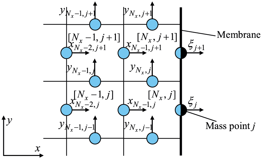
In Figure 10, the acoustic (1, 0) mode and the first mode of the membrane are dominant in the first mode, the acoustic (0, 1) mode and second mode of the membrane are dominant in the second mode, and the acoustic (1, 1) mode and second mode of the membrane are dominant in the third mode. Table 3 shows the natural frequencies of the acoustic field when all the walls are rigid, given by

$$f_a=\frac{c_a}{2}\sqrt{{\left(\frac{r}{L_x}\right)}^2+{\left(\frac{s}{L_y}\right)}^2}(r,s=0,1,2,\dots )$$

(46)

Table 3.

Natural frequency of an acoustic space when all walls are rigid.

Mode number	Natural frequency (Hz)
(0, 1)	334.17
(1, 0)	417.71
(1, 1)	534.93
(0, 2)	668.34
(1, 2)	788.14
(2, 0)	835.42

From Table 3, the natural frequency of the (1, 0) mode of the acoustic space alone is 417.71 Hz, that of the (0, 1) mode of the acoustic space alone is 334.17 Hz, and that of the (1, 1) mode is 534.93 Hz. In contrast, the natural frequency of the first mode of the coupled system, in which the (1, 0) mode of the acoustic space is dominant (Figure 10), is 283.01 Hz (Table 2). The natural frequency of the second mode, in which the (0, 1) mode of the acoustic space is dominant, is 310.32 Hz. The natural frequency of the third mode, in which the (1, 1) mode of the acoustic space is dominant, is 472.00 Hz. Therefore, the natural frequencies of the coupled problem decrease from the natural frequency of the acoustic field in the case where all walls are rigid by the coupled effect.

The numerical results obtained using the displacement model have many zero eigenvalues with a natural frequency of 0 Hz (Table 2). The variables used in the displacement model are displacements $x_{i,j}$ and $y_{i,j}$ . However, the variable used in the sound pressure model and FEM is the sound pressure $d{p}_{i,j}$ . Therefore, the cause of the zero eigenvalues is redundancy of the degree of freedom, and the number of zero eigenvalues (7821) is nearly half the degree of freedom. Figure 11 shows the mode shape of one of the zero eigenvalues by the displacement model. Figure 11(a) shows the distributions of sound pressure and membrane displacement $(N_x\times N_y=80\times 100)$ . Figure 11(b) shows one of mode shape of displacements of mass points in the acoustic space when division number is $N_x\times N_y=4\times 5$ . Each mass point in the acoustic space moves such that volume of each element does not change, and all sound pressure and displacements of the membrane are 0 in the case of zero eigenvalues. Therefore, all sound pressures and all membrane displacements are zero.

Figure 11.

Mode shape of a zero eigenvalue whose natural frequency is 0 Hz: (a) sound pressure and membrane displacement (N_x × N_y = 80 × 100) and (b) displacement in acoustic space (N_x × N_y = 4 × 5).

Figure 12 shows the natural frequency to the variation of $N_x(N_y=5N_x/4)$ . In Figure 12(a), the order of the natural frequency is first; in Figure 12(b), the order is second; and in Figure 12(c), the order is third. As the division number increases, the natural frequency by FEM approaches the convergence frequency from the higher frequency, as well known in general. On the other hand, the natural frequency by the concentrated mass model approaches the convergence frequency from the lower frequency because the concentrated mass model is similar to the lumped mass model.

Figure 12.

Natural frequency to variation of division number: (a) first order, (b) second order, and (c) third order.

Figure 13 shows the natural frequency by the concentrated mass model for first-, second-, and third-order to the variation of $L_x$ when $L_y$ is fixed $(L_y=0.5\mathrm{m})$ . The black circle shows the natural frequency at which the acoustic (0, 1) mode is dominant, as shown in Figure 10(c); the red circle shows the natural frequency at which the acoustic (1, 0) mode is dominant, as shown in Figure 10(a); and the blue circle shows the natural frequency at which the acoustic (1, 1) mode is dominant, as shown in Figure 10(e). From Figure 13, as $L_x$ increases, the natural frequency of the acoustic (1, 0) and (1, 1) dominant modes decreases. This can be explained by equation (46) when $L_x$ increases. From Figure 13, the natural frequency of the acoustic (0, 1) dominant mode does not change much because the order in the x-direction is 0 ( $r=0$ in equation (46)). Therefore, the natural frequency of the acoustic (0, 1) dominant mode overtakes that of the acoustic (1, 0) dominant mode when $L_x=0.35\mathrm{m}$ and the natural frequency of the acoustic (0, 1) dominant mode overtakes that of the acoustic (1, 1) dominant mode when $L_x=0.85\mathrm{m}$ .

Figure 13.

Natural frequency to variation of length of acoustic space in the x-direction.

Figure 14 shows the natural frequency by the concentrated mass model for first-, second-, and third-order to the variation of the membrane tension $(T_m)$ when $L_x$ and $L_y$ is fixed ( $L_x=0.4\mathrm{m}$ , $L_y=0.5\mathrm{m}$ ). The black circle shows the natural frequency at which the acoustic (0, 1) mode is dominant, the red circle shows the natural frequency at which the acoustic (1, 0) mode is dominant, and the blue circle shows the natural frequency at which the acoustic (1, 1) mode is dominant. From Figure 14, as $T_m$ increases, the natural frequency increases in each mode. The natural frequency of the acoustic (0, 1) dominant mode approaches 334.17 Hz, which is the natural frequency of the acoustic space of (0, 1) mode when all walls are rigid in Table 3. In the same way, the natural frequency of the acoustic (1, 0) dominant mode approaches 417.71 Hz and that of the acoustic (1, 1) dominant mode approaches 534.93 Hz. The widths of change of the natural frequency of the acoustic (1, 0) and (1, 1) dominant modes are larger than that of acoustic (0, 1) dominant mode because the effect of the coupling of the membrane and the acoustic (1, 0) and (1, 1) modes that have order in the x-direction is larger than the effect of the acoustic (0, 1) mode. Therefore, the natural frequency of the acoustic (1, 0) dominant mode overtakes that of the acoustic (0, 1) dominant mode when $T_m=550\mathrm{N}$ , as shown in Figure 14.

Figure 14.

Natural frequency to variation of membrane tension.

Comparison of computational time

To confirm the advantage of the proposed model over FEM, we compared the computational times for eigenvalue analysis. In the case of the displacement model or sound pressure model, the time from the decomposition in equation (25) or (30) to the acquisition of all eigenvalues is measured. In the case of FEM, the time from the calculation of the inverse matrix in equation (45) to the acquisition of all eigenvalues is measured.

Table 4 shows the computational environment. The eigenvalue analyses are performed using the Intel Math Kernel Library. The eigenvalue analysis method for the displacement model is a divide-and-conquer method for a standard symmetric eigenvalue problem; the dsyevd function of the library is used. The method for the sound pressure model is a divide-and-conquer method for a general symmetric eigenvalue problem; the dsygvd function that includes the decomposition in equation (30) is used. The method for FEM is a QR method for a standard asymmetric eigenvalue problem; the dgeev function is used. We used (20, 25), (40, 50), and (80,100) as the number of divisions ( $N_x$ , $N_y$ ) in the x- and y-directions.

Table 4.

Computational environment.

CPU	Intel Core i5-3570 CPU 3.40 GHz (4 Cores)
Memory	8.00 GB
OS	Windows 8.1 Pro (64 bit)
Compiler	Microsoft C/C++ Optimizing Compiler Version 18.00.30723
Computation library	Intel Math Kernel Library 11.1

Table 5 shows a comparison of the computational time in each division number ( $N_x$ , $N_y$ ). The sound pressure model is faster than the displacement model because it has smaller degree of freedom. The concentrated mass models (displacement model and sound pressure model) are faster than FEM because their matrices are symmetric, making them advantageous.

Table 5.

Comparison of computational times.

Nx	Ny	Concentrated mass model (displacement model)		Concentrated mass model (sound pressure model)		FEM
		DOF	Time (s)	DOF	Time (s)	DOF	Time (s)
20	25	998	0.0994	525	0.0366	570	0.3900
40	50	3960	7.498	2050	1.499	2140	13.711
80	100	15,920	491.16	8100	87.68	8280	843.30

DOF: degree of freedom.

Conclusion

To analyze the coupled problem of a two-dimensional acoustic space in a rectangular plate-shaped space and membrane vibration, we propose a concentrated mass model that consists of masses and connecting springs. The acoustic space and membrane are both modeled as a concentrated mass model. The treatment of the boundary between the acoustic space and the membrane is simply the arrangement of air masses on the membrane, so it is easy to couple the structure and acoustic field by means of the concentrated mass model. Furthermore, a sound pressure model in which sound pressure is used as the variable for the acoustic space is proposed to reduce the degree of freedom. We compared the natural frequencies of the coupled problem as obtained by the concentrated mass model (displacement model and sound pressure model) and FEM and found that they are in good agreement, and spurious modes that are physically meaningless are not generated. Furthermore, the computational times of the displacement model and sound pressure model are faster than FEM in eigenvalue analysis because its matrices are symmetric.

In summary, the proposed concentrated mass model is valid for the coupled analysis of two-dimensional acoustics and membrane vibration. Future tasks include extending this analysis to three-dimensional problems and the comparison between this method and FEM-BEM coupling method. ²⁴