
Abstract
Most contemporary high-end microphones are dynamic microphones, adopting the most basic electromagnetic transduction principles. This study investigated the diaphragm structures of dynamic microphones. The diaphragms were composed of polyimide material, and the boundary settings required for actual operation were provided using finite element model analysis software. The characteristic frequencies caused by grooving variations on the three-dimensional diaphragm were analyzed for the various groove shapes and number. The groove angles and width variations were examined based on the optimal groove shape selected in the aforementioned analysis, and the effects of these shapes were determined based on the analytical results. Acoustic waves cause thin films to vibrate, forming the working principle behind dynamic microphones. The thin film drives a coil to vibrate in a magnetic field and cuts the line of magnetic force, subsequently producing a voltage on both ends of the coil. This audio-frequency-inducted voltage represents an acoustic wave message. The finite element model analysis software was used to conduct electromagnetic induction simulations; the sound source was fed to the diaphragm to drive the coil. The coil vibrations caused the line of magnetic force to be cut, and the final voltages produced were examined and compared.
Introduction
Microphones, which are commonly known as mics (or mikes), and receivers are transducers that convert acoustic signals into electrical signals.1,2 The gramophone receiver that Edison invented in 1878 was the earliest microphone prototype. The history of the microphone can be traced to the end of the 19th century, when scientists, such as Alexander Graham Bell, searched for a favorable method to receive audio signals and enhanced the latest invention at the time, the telephone. During this period, scientists also invented the liquid and carbon microphones; however, these systems were barely usable.
In 1949, the DM4-type microphone was developed at the Wennebostel Laboratory (predecessor of the Sennheiser Laboratory) as the first feedback-suppressed, noise-compensated microphone. In 1961, Sennheiser released the MK102- and MK103-type microphones at the Hannover Industrial Fair in Germany. These two models represented a new concept for microphone fabrication: adopting compact, thin, and lightweight vibration films that guaranteed exceptional audio quality. In 1978, Sennheiser released the super-cardioid MD431-type dynamic stage microphone. This microphone provided crisp sound and a durable construction, exceptional operational noise suppression, and an integral pop filter that ensured that low-frequency stage noises would not affect the replication of sounds. During the 20th century, electro-acoustic conversion microphones evolved, initially using resistors and then inductors and capacitors. Numerous microphone technologies were gradually developed, including ribbon and dynamic microphones and the applied condenser and electret microphones, the last two of which remain widely available.3–12
Microphones collect sound in the recording link. In the earliest mechanical recorder, the microphone converted acoustic signals into diaphragm vibrations; these vibrations were then transmitted to a stylus and recorded in a series of indentations on a piece of tinfoil. Later, as magnetic recording technology evolved, microphones developed into devices that converted acoustic signals into electrical signals; these are typically classified as dynamic and condenser microphones based on their physical structures. The basic structure of a dynamic microphone10–12 comprises coils, diaphragms, and permanent magnets. When acoustic waves enter the microphone, acoustic waves pressure the diaphragm, producing vibration that moves the attached coil in the magnetic field. According to the Faraday and Lenz laws, the coils produce induction currents. The diaphragm is the core component 13 in the structure of a microphone, receiving the vibrations of acoustic waves and converting the kinetic energy into electrical signals.14,15 Dynamic microphones produce electromagnetic responses with the coils through vibration of the diaphragms. The mass of the coil requires a large acoustic pressure to drive the diaphragm, making it difficult to generate electrical signals based on the induction from subtle acoustic pressure variations. Thus, dynamic microphones are less capable of collecting subtle sounds and less sensitive compared with other microphones. Therefore, dynamic microphones are suitable for use when “detailed sounds” are not required, and because they contain coils and magnets, they exhibit multiple advantages such as sturdy materials and resistance to moisture and are unlikely to overload because of substantial acoustic pressures.
This study investigated the diaphragm structures of dynamic microphones. The diaphragms were composed of polyimide material, and the boundary settings required for actual operation were determined using finite element model (FEM) analysis software. The characteristic frequency and vibration mode were investigated in the absence of external forces. The characteristic frequencies caused by grooving variations on the three-dimensional (3D) diaphragm were analyzed for the various groove shapes and number. The groove angles and width variations were examined based on the optimal groove shape selected in the aforementioned analysis, and the effects of these shapes were determined based on the analytical results. FEM analysis software was used to conduct electromagnetic induction simulations; the sound source was fed to the diaphragm to drive the coil. The coil vibrations caused the line of magnetic force to be cut, and the final voltages produced were examined and compared.
FEM analysis of the diaphragm structure
FEM can be used to simulate various boundary conditions and dimensional changes. The COMSOL Multiphysics program comprises numerous built-in classical applied physical models and can be used to couple unlimited multiphysics quantities, coordinate sets of nonlinear partial differential equations used to solve complex numbers, and apply seamless matching layers. Thus, COMSOL FEM analysis software was used in this study to analyze microphones.
Simplified analysis of microphone vibration mode
Figure 1 shows the diaphragm model of a traditional dynamic microphone. The diaphragm is the core component in the microphone structure, receiving the vibrations of acoustic waves and converting the kinetic energy into electrical signals. The face of the dynamic microphone diaphragm receives incoming acoustic pressures, whereas the rear connects to a coil that wraps around a magnet. When the diaphragm receives incoming acoustic pressure, the diaphragm vibrates, moving the coil, which inducts electricity into the magnet. The level of acoustic pressure directly affects the diaphragm displacement, hence the inducted electrical amplitude. Because the microphone circuitry amplifies the inducted electrical current, the diaphragm displacement is a crucial factor in microphone performance.

Expanded structural diagram of a dynamic microphone.
The groove and coil parts were initially neglected when analyzing the structures of dynamic microphone diaphragms. FEM analysis software was used to provide diaphragm boundary settings during actual operation and to observe the corresponding characteristic frequencies and mode changes. Figure 2 shows a structural dimension diagram of the dynamic microphone diaphragm. The diaphragm model is disk shaped, exhibiting a diameter of 24.8 mm and a thickness of 0.019 ± 0.01 mm. The remaining unspecified tolerances were ± 0.05 mm. In this study, the vibrations of diaphragm structures that lacked groove marks were examined to observe their characteristic frequencies and mode changes. During the analytical process, the small diaphragm thickness required the use of an excessive number of solutions, causing a sluggish analysis process and yielding unsolvable conditions. To reduce the analysis time, the 3D diaphragm model was simplified into quarter circle that exhibited two-dimensional (2D) axis symmetry (Figure 3) to analyze characteristic frequencies. Furthermore, a force of 0.1 N was exerted on the diaphragm in the external excitation analysis to compare the resonant frequencies of the two models.

Schematic diagram of microphone dimensions.

Schematic diagram and boundary conditions of a 2D axis symmetrical diaphragm.
This study also performed a simplified analysis on the 3D diaphragms with grooves and subsequently compared the acoustic-solid model. Finally, the simplified model was used to analyze changes in the groove number, diaphragm thickness, and diaphragm angle.
Setting boundary conditions on the microphone diaphragm
The microphone diaphragm is composed of polyimide, and Table 1 shows the material parameters. The FEM analysis software was used to provide diaphragm boundary settings during actual operation; the outermost boundaries were fixed, and the coil-connected center was restricted to predetermined displacement directions (Figure 3). The simplified models exhibited a quarter circle and 2D axis symmetry. The original disk-shaped diaphragm was simplified into a quarter circle to analyze the characteristic frequencies at one-fourth of the original size, reducing the analysis time. Thus, symmetry plane settings were assigned to the disk division boundaries, whereas the remaining settings remained identical to those of the original model. The upper surface of the diaphragm was assigned a load of 0.1 N in the external excitation analysis to observe the variation in resonant frequencies.
Material parameters of polyimide and copper.

The boundary conditions of the grooved diaphragms were identical to those of the original model. The acoustic-shell coupling module of the software was used to analyze the effects of varying groove angles and widths. This model initially provided component displacements, simulating model variations as sounds reached the component. Thus, preliminary displacement boundary conditions were assigned to the coil-connected center of the diaphragm. The boundary conditions differed from the preliminary displacement conditions provided by the diaphragm shape variation analysis. Here, the preliminary displacement required a coordinate in the z-direction. The material outside the spherical region was set as air, and the boundaries were set as spherical radiation.
Mesh planning in FEMs
The excessively thin microphone diaphragm exacerbated the FEM software meshing process; thus, mesh divisions were separated into two parts: mapped and free tetrahedral meshing. Given identical unit edge lengths, mapped meshing produces substantially smaller mesh sizes compared with free meshing, requiring fewer computation resources, speeding the computation process, and typically yielding superior precision. Because grooved diaphragm models are complex and 3D mapped meshing on them is difficult, free tetrahedral meshing was adopted to divide the models.
Mapped meshing is primarily used to divide 2D models into tetrahedrons. The boundaries of the quarter disk models were initially divided into two dimensions. The mesh grids were then rotated 90° to complete mesh planning for the simplified quarter models. The mesh planning for the original full-disk model was identical to that of the quarter disk models. Because the 2D axis symmetry is a 2D model, only the mapped meshing boundary needed to be divided, and mesh rotation was disregarded.
In this study, free tetrahedral meshing was employed in a simplified shell analysis. Tetrahedral meshing is suited for use in free meshing and can be rapidly and automatically generated. Curvature and approximate dimensional functions were used to refine the mesh sizes in key regions. The grooved models were complex and excessively thin, increasing the difficulty of mesh division. Frequency response and characteristic frequency analyses were conducted to assess the variations in groove number. Thin-shell models were adopted in the characteristic frequency analyses. The groove shapes of the thin shells yielded dense mesh grids, and the grid planning of the leaf slots was relatively more evenly meshed. Acoustic-shell coupling analysis was adopted to assess the frequency responses. This module involved a spherical region around the diaphragm model. Thus, the mesh sizes differed according to the diaphragm and sphere regions.
Simplified analysis of nongrooved diaphragm
Heavy computations yield prolonged analyses; therefore, the 3D disk diaphragm model was simplified to avoid unsolvable conditions. Because the diaphragm is intrinsically a symmetrical structure, the 3D 360° model can be reduced to a 90° quarter sphere model. The 2D axis symmetry was employed for the simplified module to simulate the operating conditions of the diaphragm and elucidate the characteristic values and mode changes in the absence of external excitation. The characteristic frequencies of the nonsimplified, quarter disk, and 2D axis symmetrical diaphragms were 867, 866, and 861 Hz, respectively; the differences among these characteristic frequencies were within the margin of error.
External excitation analyses were also performed on the quarter disk and 2D axis symmetrical models by exerting a load of 0.1 N on the diaphragm surfaces and performing a frequency sweep at every 1 Hz within the sweep range of 500–1000 Hz. The results indicated that the first resonant frequencies of the 2D axis symmetry and quarter disk were 862 and 868 Hz, respectively. Most people speak in the frequency range of 100–10,000 Hz. Both results were within the vocal range and margin of error, verifying that simplified models can be used for disk-shaped diaphragms. Moreover, the calculated results showed that the external excitation analyses took 4–5 min when assessing the 2D axis symmetry but 12 days when assessing the quarter disk models. Thus, after comparing and verifying the simplified models, the results indicated a substantial reduction in the analysis times.
Simplified analysis of 3D grooved diaphragm
Based on the results in the previous section, nongrooved diaphragms can be simplified to 2D axis symmetry, but incorporated grooves introduce nonsymmetry to the model due to their groove angles. Thus, grooved diaphragms cannot be simplified using 2D axis symmetry. However, commercially available diaphragms typically receive additional surface fabrication to enhance their durability and suppleness. The 3D grooved diaphragm models yield comparatively more detailed analyses but require prolonged computation times. Therefore, the thin-shell element in the solid mechanics module was used to conduct a simplified analysis of 3D grooved diaphragms.
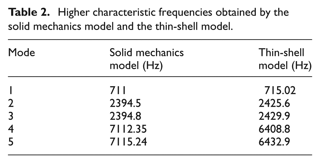
According to the thin-shell module, the diaphragm is viewed as a thin shell (Figure 4(b)). Because the thickness dimensions were separately entered, the diaphragm had no thickness restrictions in this module. The boundary settings were similar to those of the previous diaphragm settings. To prove the feasibility of conducting simplified thin-shell diaphragm analyses, structural mechanics (Figure 4(a)) were employed, using the solid mechanics module to analyze and compare the simplified and nonsimplified 3D grooved diaphragms. The results indicated that the first characteristic frequencies for the simplified and nonsimplified grooved diaphragms were about 715 and 711 Hz, respectively. The differences in the first characteristic frequency were minimal, and the deformations were almost consistent; thus, using thin-shell simplified analysis can reduce the required computation time. Table 2 shows the higher characteristic frequencies obtained by the solid mechanics model and the thin-shell model to verify the efficiency of the thin-shell model.
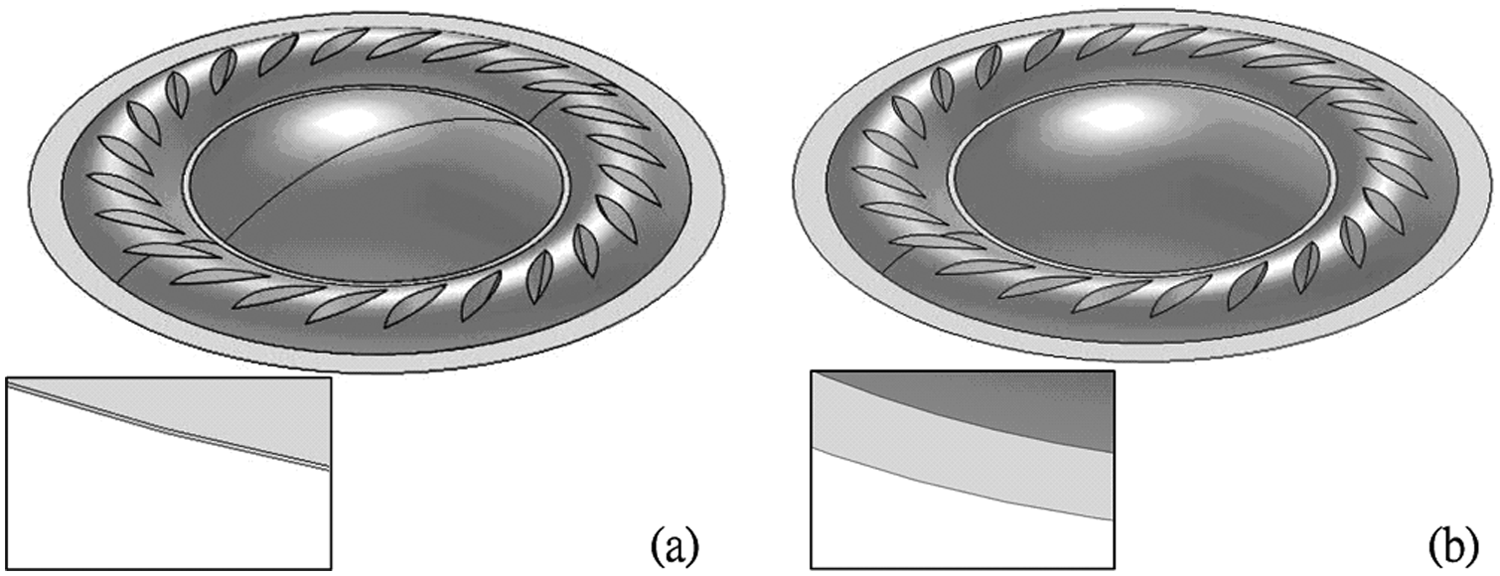
(a) Thickness schematic diagram of a solid-state mechanical model and (b) thickness of a thin-shell model.
Higher characteristic frequencies obtained by the solid mechanics model and the thin-shell model.
Effect of groove shape and number on the diaphragm
Multiple frequency response parameters affect the microphone diaphragm, including Young’s modulus, density, formation temperature, and thermal expansion coefficient. Theoretical equations can be used to estimate how most of these parameters affect the characteristic frequencies of the diaphragm; however, analyzing how adding several grooves affects the characteristic frequencies requires using FEM analyses to acquire information regarding trend changes. Two groove shapes were simulated in this study. First, leaf-slot-shaped grooves were analyzed in sets of 4, 12, 24, and 32. Subsequently, grooves were analyzed in sets of 1, 3, 5, and 7. The results of these shapes were compared by observing trends caused by an increasing number of grooves. Figures 5 and 6 show the diaphragm dimensions when using leaf slots and groove-like diaphragms, respectively.

Structural diagram of the leaf-slot diaphragm.

Structural dimensions of the grooved diaphragm.
Effect of groove shape and number on characteristic frequency
The characteristic frequencies of diaphragms were examined using sets of 4, 12, 24, and 32 leaf slots. The first characteristic frequency that lacked grooves yielded 829 Hz. Adding four leaf slots decreased the first characteristic frequency to 742 Hz. Then, as the number of leaf slots added increased, the first characteristic frequencies of the grooved diaphragms gradually decreased. In addition, the characteristic frequencies were analyzed using 1, 3, 5, and 7 sets of grooves. The first characteristic frequency decreased from 852 to 821 Hz when the first groove was added to a nongrooved diaphragm; subsequently, the first characteristic frequency rebounded to 827 Hz when three grooves were added. This upward trend increased to a peak value of 854 Hz at five grooves and then declined when the groove number increased to seven. Tables 3 and 4 show the effect of the leaf slots and groove number on the characteristic frequencies.
Effect of leaf slot number on the characteristic frequencies.

Effect of groove number on the characteristic frequencies.

Effect of groove shapes and numbers on frequency responses
The characteristic frequency analysis was used to study the frequency response effect by increasing the groove number. An acoustic-shell coupling module was employed in the frequency response analysis. The acoustic-shell coupling module can simulate thin elastic structural vibrations, induce acoustic pressure fields, and couple the diaphragm with the acoustic field using shell simplification. A sound source point was established at an output of 1 W to analyze the frequency response from 20 Hz to 20 kHz.
Frequency response refers to the amplification and attenuation of the output signal based on the frequency changes as the microphone receives various sound signals. The comparative results for the nongrooved, leaf-slot, and grooved diaphragms when the normal field obtained using the frequency response analysis were displaced in the z-direction. The displacement results of nongrooved diaphragms showed that other than the few primary excitation points, numerous sporadic excitation points were observed in the mid-to-high frequency. An increased number of leaf slots yielded increased flatness in the frequency response normal field displacements, particularly when 24 leaf slots were evaluated. By contrast, an increased number of grooves did not yield increased flatness in the frequency displacement curves but rather increased the sporadic excitation points in the mid-to-high frequencies.
The most favorable acoustic pressure curves are smooth curves, which indicate that the output signals realistically represent the characteristics of the original sound; however, such conditions are not easily attained. The horizontal axis in the frequency response represents the frequency in Hertz and is typically expressed in logarithmic terms. The vertical axis represents the level of acoustic pressure in decibel. Figure 7(a) shows the result of the acoustic pressure curve in the frequency response investigation. Obvious fluctuation points occurred in the mid-to-high frequency regions of the acoustic pressure curves for the nongrooved diaphragm. The acoustic pressure curves became increasingly smooth as the number of leaf slots increased in the leaf-slot diaphragms, particularly when 24 leaf slots were evaluated as shown in Figure 7(b); however, the acoustic pressure curves became increasingly unstable in the high frequency region as the number of grooves increased in the grooved diaphragms as shown in Figure 7(c).

Frequency response diagram of (a) a nongrooved diaphragm, (b) a 24 leaf-slot diaphragms, and (c) a 7-grooved diaphragm.
Angle and width variation analysis of leaf-slot diaphragms
In this study, the variations of leaf angles and thicknesses of the superior leaf-slot diaphragms underwent a change analysis. The leaf slots were divided into widths of 0.4, 0.8, and 1.0 mm (Figure 8). Models using each width were then assigned to various leaf angles that varied in 5° increments between 0° and 45°. First, the characteristic frequency of each model was analyzed. Subsequently, the first characteristic frequencies of the analysis were plotted and compared (Figure 9). When 0.8 mm was used as a basis for leaf slot width, the graph indicated that the first characteristic frequencies at 1.0 mm typically decreased; by contrast, the first characteristic frequencies typically increased at 0.4 mm. The vibration modes and characteristic frequencies of the diaphragm can be acquired by conducting a characteristic frequency analysis. Thus, the first modal characteristic frequency was observed at approximately 800 Hz, which is optimal for use in general vocal applications.

Width variation of leaf-slot diaphragms: (a) 0.4, (b) 0.8, and (c) 1.0 mm.

Frequency trend of leaf angle variations.
The frequency domains of various leaf widths and leaf angles were analyzed using acoustic-shell coupling modules. According to these acoustic-shell coupling modules, the diaphragm is primarily viewed as a thin shell, and an outer spherical region was added as air. The boundaries were set similarly to those in the previous diaphragm models. The coil-connected centers were set using predetermined displacement restrictions on the x- and y-axes; each set of the sound source was given a value of 1 W, and the analytic solver frequencies were set at 800 Hz and 1 kHz. Two frequencies were selected primarily because the 800-Hz frequency range influenced the sound intensity. At this frequency, fullness yields powerful sounds; conversely, shortages at this frequency cause flaccid sounds. In other words, low-frequency components become more apparent for frequencies below 800 Hz. Furthermore, 1 kHz is the standard reference frequency used in audio equipment testing. A preliminary investigation into the displacement variations in the frequency domains indicated that the magnitude of displacement increased as the angle increased. The results demonstrated that characteristic frequencies exhibiting a width of 0.4 mm and an angle of 45° were similar to the 800-Hz model and that the model displacement was the largest among all models. In the frequency domain of 1 kHz, the displacement exhibiting a width of 0.8 mm and an angle of 45° was most similar to that exhibited at a width of 0.4 mm and an angle of 45°. By contrast, the first characteristic frequencies acquired using a 1-mm leaf width were typically lower compared with those acquired using other leaf widths. In addition to an increased displacement variation at 0°, the results indicated no major fluctuations at the other leaf angles.
Electromagnetic induction analysis of the dynamic microphone
Numerous types of microphones exist, and this study focused on dynamic microphones. The principle of dynamic microphones is using a sound source to vibrate the diaphragm; this vibrates the coil in the magnetic field, inducing a voltage. The amount of voltage induced changes as the volumes and frequencies of the sound source change. Dynamic microphones are composed of coils and permanent magnets, producing voltage based on Fleming’s left hand rule. This study analyzed the coupling of electric fields, acoustic fields, and structural mechanics. To reduce the time and memory spent on analyses, 2D axis symmetry was adopted in the electromagnetic and structural mechanic analyses. The electromagnetic results were subsequently imported into a 3D model to avoid generating unsolvable conditions because of heavy computations when using the FEM analysis software.
Electromagnetic induction analysis of the 2D axis symmetry
Four application modules were used in the electromagnetic induction analysis of the 2D axis symmetry: a quasi-static magnetic module in the AC or DC module, a piezoelectric axis symmetry and acoustic pressure module in the acoustic field module, and, finally, an axis symmetry stress–strain module in the structural mechanic module. The quasi-magnetic module was used to compute the magnetic field distribution of the permanent magnet and determine the magnetic force (BL). An acoustic wave was then simulated using the piezoelectric axis symmetry module; its force was exerted on the diaphragm using the air domain and perfectly matched layer (PML) of the acoustic module. Finally, the BL were introduced and coupled to the structural mechanic module to determine the induction voltages. Figure 10 shows the 2D axis symmetry analysis model.
Schematic model of the 2D axis symmetry.
Electromagnetic analysis of the 2D axis symmetry
The rendered drawing files (Figure 11) were introduced to the quasi-static magnetic module and then entered using the dynamic microphone constants as shown in Table 5. The upper and lower pole piece materials were set as iron, and the permanent magnets were set using a residual magnetic flux for the subdomain settings. Next, integration coupling variables were set for the coils as follows


Dimensional schematic representation of a 2D axis symmetrical model.
Dynamic microphone constants.

where Br is the magnetic flux density, N is the coil turns, and A is the coil cross-sectional area.
Here, the model was divided using free mesh parameters. Regarding the subdomain settings, the maximal mesh elements of the upper and lower pole pieces and permanent magnets were set at 1 × 10⁻³ mm. Finally, the BL was determined.
Acoustic-solid coupling analysis of the 2D axis symmetry
A piezoelectric crystal plate was adopted in the acoustic-solid coupling analysis to simulate an acoustic wave. When the air domain acted on the diaphragm, it produced diaphragm–coil displacement. Regarding the subdomain settings, PZT-5H was used as the piezoelectric crystal plate material, and copper and polyimide were used as the coil and diaphragm materials, respectively (Table 1). The constants were imported with the BL determined using the electromagnetic analysis (Table 5). The scalar expressions were set using the induction electromagnetic force (EMF; Vi) equation as shown in Table 6. The frequency range of 20 Hz–2 kHz was solved following the air region and PML settings.
Scalar expression of dynamic microphones.

Electromagnetic induction analysis of the 2D axis symmetry
Because of the diaphragm weight gain caused by adding the coil, the resonant frequency of the dynamic microphone decreased to approximately 160 Hz. The BL was imported for coupling to determine the induction EMF (Vi). When the externally provided resonant frequency was identical to that of the intrinsic resonant frequency of the diaphragm design structure, the diaphragm was subjected to the largest displacement; this indicates that the coil exhibited the largest magnetic flux variation. The magnitude of the induction EMF was absolutely related to the swing of the amplitude. A large swing yielded a correspondingly large EMF, indicating that increased resonant frequencies yield increased structural electric generation.
In dynamic microphones, voltage generation is primarily based on Fleming’s left hand rule. The results of the 2D axis symmetry analysis demonstrate magnetic field variations. When the diaphragm was subjected to an acoustic wave, producing downward displacement, an opposite force was produced against the coil to prevent it from entering the magnetic field of the permanent magnet and to sustain the electroneutrality of the coil loop (Figure 12). In other words, magnetic field variation produced an induction current, which generated a force in the magnetic field to counter the magnetic field variation. By contrast, as the diaphragm returned and the coil became displaced upward when the acoustic wave stopped, the magnetic field generated by the induction currents prevented the coil from returning because of the remnant magnetic field in the coil generated by the permanent magnet (Figure 13). This phenomenon is known as Lenz’s Law.

Transient magnetic field diagram as the coil approaches the permanent magnet.

Transient magnetic field diagram as the coil withdraws from the permanent magnet.
3D acoustic-shell module induction EMF simulation analysis
Because of the difficulties in incorporating grooves in the 2D axis symmetrical models, a 3D partial analysis was adopted using the acoustic-shell module; however, simulating electromagnetic induction is a coupled problem. To conserve central processing unit time and memory use, the electromagnetic section was simulated using 2D axis symmetry and subsequently imported into the 3D model to avoid unsolvable conditions caused by heavy computations. Electrical resistance and impedance were initially neglected in this section.
The frequency responses of grooved diaphragms were analyzed and compared with the results of a 2D axis symmetry analysis to verify the feasibility of using the 3D acoustic-shell module; subsequently, the leaf-slot diaphragms were analyzed. The frequency response range was set from 100 Hz to 2 kHz in 10-Hz increments. In addition, sound source was provided for the diaphragm, using a time-dependent analysis set to a range of 0–1 s in 0.01-s increments.
Boundary settings of the acoustic-shell module analysis
Simulating electromagnetic induction must address the coil effect. The diaphragm can be simplified in the acoustic-shell module during analysis, but the coil cannot be analyzed as a simplified thin shell. Therefore, the coil boundaries were set with an increased copper mass of 1.85403 × 10⁻⁴ kg in the diaphragm.
3D induction EMF frequency-domain simulation
The resonant frequency of the nongrooved diaphragm in the acoustic-shell module was approximately 170 Hz, which was similar to the result for the 2D axis symmetrical model. Regarding displacement, the results varied because distinct external force modes were applied to the simulation model. This verified that the acoustic-shell module could be simulated using an attached coil. The frequency responses of the diaphragm that exhibited 24 leaf slots and a 45° leaf angle were subsequently analyzed. The results indicated that an increased number of leaf slots decreased the resonant frequency of the diaphragm to approximately 130 Hz. Although the resonant frequency of the diaphragm decreased as the number of leaf slots increased, the increased diaphragm suppleness produced increased displacement.
The diaphragm velocities (v) were generated by conducting a frequency analysis of the nongrooved and leaf-slot diaphragms, multiplied by the BL, to determine the induction EMF, ε = −Blv. Dividing the induction EMF by the coil resistance yields the corresponding induction current

Induction current diagram of the frequency response analysis.
3D induction EMF simulation time dependency
A sound source was provided for the diaphragm during the time dependency analysis to simulate the actual conditions when the diaphragm received sounds. A time-dependent analysis was conducted from 0 to 1 s at 0.01- s increments, and the results were further investigated. The settings were identical to those used in the frequency-domain analysis. Nongrooved and 24-groove diaphragms were analyzed, and their velocities were determined based on the integrated displacements (Figure 15). Finally, the velocities were used to compute the induction EMFs and currents.

Diaphragm velocity diagram.
Figures 16 and 17 show the induction EMF and current trends produced by the nongrooved and 24-groove diaphragms after receiving a signal, indicating that nongrooved diaphragms produce less stable induction EMF compared with 24-groove diaphragms; by contrast, the 24-groove diaphragms produced more stable induction EMF compared with the nongrooved diaphragms. Regarding the induction current, the nongrooved diaphragm produced the largest induction current in the final segment of the analytical time, but the 24-groove diaphragm produced the most stable current within the analytical time. Overall, the 24-groove diaphragms were less satisfactory compared with the nongrooved diaphragms.

Induction EMF diagram of the diaphragms.

Induction current diagram of the diaphragms.
Conclusion
Dynamic microphones use electromagnetic induction to produce an output signal. This principle involves generating a specific energy and directional current when a conductive metallic coil passes through a magnetic field line. Thus, it is critical to assess how diaphragm displacement affects dynamic microphones. In this study, analyses were conducted using the COMSOL Multiphysics software suite. To conserve the time and computational effort spent on analyses, several simplification analyses and verifications were conducted to rapidly and accurately obtain results. In addition, this study focused on the various shapes, numbers, and angles of diaphragm grooves, determining the optimal design parameters for conducting electromagnetic induction analyses.
Footnotes
Academic Editor: Luís Godinho
Declaration of conflicting interests
The authors declared no potential conflicts of interest with respect to the research, authorship, and/or publication of this article.
Funding
This study was supported by the Ministry of Science and Technology of Taiwan (project no. NSC 101-2628-E-150-001-MY3).