Massively parallel least squares finite element method with graphic processing unit

Abstract

For the reason of enormous computational expense, although the least squares finite element method has the advantages of high accuracy, robustness and strong versatility, the application of it is limited in computational fluid dynamics. The problems solved in this article include the rewriting of branching statements and the kernel function, variable distribution and data transfer between graphic processing units, and library functions rewriting. To the best knowledge of the authors, this article is the first time to develop the parallel computing codes for single and multiple graphic processing units based on the least squares finite element method. The computational results of single and multiple graphic processing units are verified by lid-driven cavity flow. Compared with a single central processing unit on the condition of 120³ grids, the acceleration ratios of single and dual graphic processing units are up to 70.5 times and 95.2 times, respectively, which is much higher than the previous value of 7.7. With the increase in the grid number, the acceleration ratio of single and multiple graphic processing units is expected to increase, which can greatly enhance the computational efficiency of the least squares finite element method. Therefore, it is possible to solve the massive turbulence computing by the least squares finite element method with higher efficiency.

Introduction

Finite element method, finite difference method and finite volume method are the main methods of computational fluid dynamics (CFD). In the past three decades, Jiang ¹ and Bochev and Gunzburger ² have developed the least squares finite element method (LSFEM) by combining the least squares method and the finite element method. LSFEM has been applied initially in the field of incompressible flow by Ding and Tsang ³ and Tang and Sun, ⁴ thermodynamics by Zhao et al. ⁵ and Luo et al. ⁶ and fluid–structure interaction by Kayser-Herold and Matthies. ⁷

LSFEM has the advantages of good convergence, good universality, good robustness and high accuracy. However, it requires a lot of computational expense, which can lead to long computational time, thus restricting the application in turbulent flow problems. Turbulent flow problems have large computational amount and complicated flow structure. In order to shorten the computational time and solve more complex turbulence problems, Ding et al. ⁸ developed a large-scale parallel computing of LSFEM by message passing interface (MPI) on the central processing unit (CPU) platform, which obtained acceleration ratio of 7.7.

The graphic processing unit (GPU) can be thought as a massively parallel computer with several hundred cores, in which several hundred to thousands of threads that execute instructions in parallel. Due to the powerful processing power and high bandwidth, GPU has a significant advantage in computational cost, which outperforms the ability of CPU. Vanka ⁹ reviews the literature of linear solvers and CFD algorithms based on GPUs. He pointed out that several researchers have developed/ported CFD software to GPUs and founded significant speedups (10–50 times, depending on algorithm, approach and implementation) over a single-core CPU.^10–12 Although computing unified device architecture (CUDA) reduces the difficulty of GPU general-purpose computing, porting existing CPU codes to run on the GPU requires the user to write kernels that execute on multiple cores, which hinders the use of researchers. In order to achieve semi-automatic or fully automatic from CPU to GPU, Corrigan and Lohner ¹³ and Chandar et al. ¹⁴ developed a semi-automatic technique and CU++, respectively. The semi-automatic technique simultaneously achieves the fine-grained parallelism required to fully exploit the capabilities of multi-core GPUs, completely avoids the crippling bottleneck of GPU–CPU data transfer and uses a transposed memory layout to meet the distinct memory access requirements posed by GPUs. CU++ uses object-oriented programming techniques available in C++ and allows a code developer with just C/C++ knowledge to write computer programs that will execute on the GPU without any knowledge of specific programming techniques in CUDA because CUDA kernels is generated automatically during compile time.

To the best knowledge of the authors, above applications on the GPU platform did not involve LSFEM. GPU acceleration for LSFEM computation could be a new choice. The author has been engaged the GPU parallel computing of dissipative particle dynamics, of which the speedup ratio is about 20 times compared with CPU serial computing. ¹⁵ Based on previous researches on LSFEM, this article developed CFD codes for single GPU and dual GPUs. By comparing the flow result and acceleration ratio of lid-driven cavity flow between GPU calculation and single CPU calculation, the feasibility and accelerated performance of GPU computation for LSFEM are evaluated. The structure of this article is as follows: Introduction of LSFEM; Code framework for single GPU and dual GPUs; Acceleration ratio of GPU computation and CPU computation; and Conclusion.

Least squares finite element method

LSFEM belongs to the category of finite element method, based on weighting residual method. This method uses residual as weighting functions to calculate inner product of residuals. In solving flow problems, it can get a symmetrical positive-definite coefficient matrix, which is easy and effective to solve mathematically. The authors first developed vorticity and stress formulations of LSFEM to solve Navier–Stokes (N-S) equations ¹⁶ and then developed large eddy simulation to solve turbulence flow. ¹⁷ All developed CFD codes are single precision CPU codes and can be paralleled. However, the degree of parallelism is not high and the efficiency is low, which leads to high computation time and cost in turbulence calculation.

Incompressible non-dimensional N-S equations in the form of stress tensor are presented as follows

$$\begin{array}{c}\frac{\partial u_j}{\partial x_j}=0\hfill \\ \multicolumn{1}{c}{\frac{\partial (u_i{u}_j)}{\partial x_j}+\frac{\partial p}{\partial x_i}-\frac{2}{\mathrm{Re}}\frac{\partial S_{\mathrm{ij}}}{\partial x_j}=f_i}\\ S_{\mathrm{ij}}=\frac{1}{2}(\frac{\partial u_i}{\partial x_j}+\frac{\partial u_j}{\partial x_i})\hfill \end{array}$$

(1)

where u is the velocity, p is the pressure, S_ij is the stress tensor, f is the volume force and Re is Reynolds number.

For two-dimensional (2D) flow, the non-linear convective term in equation (1) is linearized by Newtonian method and equation (2) can be obtained. u₀ and v₀ in equation (2) are usually given the initial value of zero

$$\begin{array}{c}\frac{\partial u}{\partial x}+\frac{\partial v}{\partial y}=0\hfill \\ u_0\frac{\partial u}{\partial x}+v_0\frac{\partial u}{\partial y}+u\frac{\partial u_0}{\partial x}+v\frac{\partial u_0}{\partial y}+\frac{\partial p}{\partial x}\hfill \\ -\frac{2}{\mathrm{Re}}(\frac{\partial S_{11}}{\partial x}+\frac{\partial S_{12}}{\partial y})=f_x+u_0\frac{\partial u_0}{\partial x}+v_0\frac{\partial u_0}{\partial y}\hfill \\ u_0\frac{\partial v}{\partial x}+v_0\frac{\partial v}{\partial y}+u\frac{\partial v_0}{\partial x}+v\frac{\partial v_0}{\partial y}+\frac{\partial p}{\partial y}\hfill \\ -\frac{2}{\mathrm{Re}}(\frac{\partial S_{12}}{\partial x}+\frac{\partial S_{22}}{\partial y})=f_y+u_0\frac{\partial v_0}{\partial x}+v_0\frac{\partial v_0}{\partial y}\hfill \\ S_{11}-\frac{\partial u}{\partial x}=0\hfill \\ S_{12}-\frac{1}{2}(\frac{\partial u}{\partial y}+\frac{\partial v}{\partial x})=0\hfill \\ S_{22}-\frac{\partial v}{\partial y}=0\hfill \end{array}$$

(2)

The corresponding vectors and matrix are shown in equation (3), where subscript 0 denotes the result from previous iteration

$$\mathit{u}=(\begin{array}{cccccc}\hfill u\hfill & \hfill v\hfill & \hfill p\hfill & \hfill S_{11}\hfill & \hfill S_{12}\hfill & \hfill S_{22}\hfill \end{array}{)}^T$$

(3)

$${\mathit{A}}_0=\left(\begin{array}{cccccc}\hfill 0\hfill & \hfill 0\hfill & \hfill 0\hfill & \hfill 0\hfill & \hfill 0\hfill & \hfill 0\hfill \\ \multicolumn{1}{c}{\frac{\partial u_0}{\partial x}}& \hfill \frac{\partial u_0}{\partial y}\hfill & \hfill 0\hfill & \hfill 0\hfill & \hfill 0\hfill & \hfill 0\hfill \\ \multicolumn{1}{c}{\frac{\partial v_0}{\partial x}}& \hfill \frac{\partial v_0}{\partial y}\hfill & \hfill 0\hfill & \hfill 0\hfill & \hfill 0\hfill & \hfill 0\hfill \\ \multicolumn{1}{c}{0}& \hfill 0\hfill & \hfill 0\hfill & \hfill 1\hfill & \hfill 0\hfill & \hfill 0\hfill \\ \multicolumn{1}{c}{0}& \hfill 0\hfill & \hfill 0\hfill & \hfill 0\hfill & \hfill 1\hfill & \hfill 0\hfill \\ \multicolumn{1}{c}{0}& \hfill 0\hfill & \hfill 0\hfill & \hfill 0\hfill & \hfill 0\hfill & \hfill 1\hfill \end{array}\right){\mathit{A}}_1=\left(\begin{array}{cccccc}\hfill 1\hfill & \hfill 0\hfill & \hfill 0\hfill & \hfill 0\hfill & \hfill 0\hfill & \hfill 0\hfill \\ \multicolumn{1}{c}{u_0}& \hfill 0\hfill & \hfill 1\hfill & \hfill -\frac{2}{\mathrm{Re}}\hfill & \hfill 0\hfill & \hfill 0\hfill \\ \multicolumn{1}{c}{0}& \hfill u_0\hfill & \hfill 0\hfill & \hfill 0\hfill & \hfill -\frac{2}{\mathrm{Re}}\hfill & \hfill 0\hfill \\ \multicolumn{1}{c}{-1}& \hfill 0\hfill & \hfill 0\hfill & \hfill 0\hfill & \hfill 0\hfill & \hfill 0\hfill \\ \multicolumn{1}{c}{0}& \hfill -0.5\hfill & \hfill 0\hfill & \hfill 0\hfill & \hfill 0\hfill & \hfill 0\hfill \\ \multicolumn{1}{c}{0}& \hfill 0\hfill & \hfill 0\hfill & \hfill 0\hfill & \hfill 0\hfill & \hfill 0\hfill \end{array}\right){\mathit{A}}_2=\left(\begin{array}{cccccc}\hfill 0\hfill & \hfill 1\hfill & \hfill 0\hfill & \hfill 0\hfill & \hfill 0\hfill & \hfill 0\hfill \\ \multicolumn{1}{c}{v_0}& \hfill 0\hfill & \hfill 0\hfill & \hfill 0\hfill & \hfill -\frac{2}{\mathrm{Re}}\hfill & \hfill 0\hfill \\ \multicolumn{1}{c}{0}& \hfill v_0\hfill & \hfill 1\hfill & \hfill 0\hfill & \hfill 0\hfill & \hfill -\frac{2}{\mathrm{Re}}\hfill \\ \multicolumn{1}{c}{0}& \hfill 0\hfill & \hfill 0\hfill & \hfill 0\hfill & \hfill 0\hfill & \hfill 0\hfill \\ \multicolumn{1}{c}{-0.5}& \hfill 0\hfill & \hfill 0\hfill & \hfill 0\hfill & \hfill 0\hfill & \hfill 0\hfill \\ \multicolumn{1}{c}{0}& \hfill -1\hfill & \hfill 0\hfill & \hfill 0\hfill & \hfill 0\hfill & \hfill 0\hfill \end{array}\right)\mathit{f}=\left(\begin{array}{c}\hfill 0\hfill \\ \multicolumn{1}{c}{f_x+u_0\frac{\partial u_0}{\partial x}+v_0\frac{\partial u_0}{\partial y}}\\ \multicolumn{1}{c}{f_y+u_0\frac{\partial v_0}{\partial x}+v_0\frac{\partial v_0}{\partial y}}\\ \multicolumn{1}{c}{0}\\ \multicolumn{1}{c}{0}\\ \multicolumn{1}{c}{0}\end{array}\right)$$

Using finite element analysis, the computational domain is discretized into many sub-regions, where the unknown quantities are

$${\mathit{u}}^e=\sum _{j=1}^{N_n}{\psi }_j(x)(\begin{array}{cccccc}\hfill u\hfill & \hfill v\hfill & \hfill p\hfill & \hfill S_{11}\hfill & \hfill S_{12}\hfill & \hfill S_{22}\hfill \end{array}{)}_j^T$$

(4)

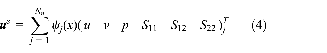
where N_n is node number of sub-region, ψ _j is the shape function of each node.

According to finite element method, the final form is then as

$$\mathit{KU}=\mathit{F}$$

(5)

where K is global stiffness matrix, U is global unknown vector, which is formed by the unknown quantities of each node u ^e , and F is the known vector.

The global stiffness matrix and known vector are formed by the stiffness matrix and known quantities of node, respectively. According to the theory of least square method, the stiffness matrix of node K_e and known quantities of node Fe are shown as equations (6) and (7), respectively, with Aψ_j given as equation (8)

$${\mathit{K}}_e={\displaystyle \int {(\mathit{A}{\psi }_1,\mathit{A}{\psi }_2,\dots ,\mathit{A}{\psi }_{N_n})}^T●(\mathit{A}{\psi }_1,\mathit{A}{\psi }_2,\dots ,\mathit{A}{\psi }_{N_n})d\Omega }$$

(6)

$${\mathit{F}}_e=\int {(\mathit{A}{\psi }_1,\mathit{A}{\psi }_2,\dots ,\mathit{A}{\psi }_{N_n})}^{\mathrm{T}}\mathit{f}\mathrm{d}\mathrm{\Omega }$$

(7)

$$\mathit{A}{\psi }_j={\mathit{A}}_1\frac{\partial {\psi }_j}{\partial x}+{\mathit{A}}_2\frac{\partial {\psi }_j}{\partial y}+{\mathit{A}}_0{\psi }_j$$

(8)

It is important to point out that K is positive-definite matrix, which can be solved by the efficient method of conjugate gradient. Jacobi preconditioned conjugate gradient (JPCG), which can be referred to Jiang, ¹ was used to solve the equations above. Q , diagonal matrix of K , was chosen as the preconditioned matrix. The iterative steps are as follows.

Pick arbitrary initial vector U ⁰, calculate

$${\mathit{R}}^0=\mathit{F}-\mathit{K}{\mathit{U}}^0={\mathit{P}}^0$$

(9)

$${\mathit{B}}^0={\mathit{Q}}^{-1}{\mathit{R}}^0$$

(10)

For i = 0, 1, …, n − 1, iterate

$$a_i=\frac{({\mathit{B}}^i,\mathit{Q}{\mathit{R}}^{\mathit{i}})}{({\mathit{P}}^{\mathit{i}},\mathit{K}{\mathit{P}}^{\mathit{i}})}$$

(11)

$${\mathit{U}}^{\mathit{i}+1}={\mathit{U}}^{\mathit{i}}+a_i{\mathit{P}}^{\mathit{i}}$$

(12)

$${\mathit{B}}^{n+1}={\mathit{B}}^n+a_i{\mathit{Q}}^{-1}\mathit{K}{\mathit{P}}^0$$

(13)

$${\beta }_i=\frac{({\mathit{B}}^{\mathit{i}+1},\mathit{Q}{\mathit{B}}^{\mathit{i}+1})}{({\mathit{B}}^{\mathit{i}},\mathit{Q}{\mathit{B}}^{\mathit{i}})}$$

(14)

$${\mathit{P}}^{i+1}=R^{i+1}-{\beta }_i{\mathit{P}}^i$$

(15)

Iteration stops when R ⁱ is small enough to be seen as convergence. The codes are as follows:

• Itro = 0

• do {    //outer loop

•  itro = itro + 1;

•  itri = 0;

•  boundary condition for initialization of U[ ]

•  D[ ] = U[ ];

•  KD[ ] = Kmly(D[ ]);   //Kmly(D[ ]) for K ×D[ ]- Fcompatible with equation (9)

•  Q[ ] = Kdiag( );   //Kdiag( ) for diagonal matrix of K

•  R[ ] = -pn[ ];

•  D[ ] = R[ ]/Q[ ];   //compatible with equation (10)

•  do { //inner loop

•  itri = itri + 1;

•  KD[ ] = Kmly(D[ ]);

•  d0 = (R[ ], R[ ]/Q[ ]);

•  t = d0 / (D[ ], KD[ ]);    // compatible with equation (11)

•  U[ ] = U[ ] + t*D[ ];    //compatible with equation (12)

•  R[ ] = R[ ]-t* KD[ ];    //compatible with equation (13)

•  d1 = (R[ ], Q[ ]);    //compatible with equation (14)

•  alpha = d1/d0;

•  D[ ] = R[ ]/Q[ ] + alpha*D[ ];.    // compatible with equation (15)

•  r2 = |R[ ]|^2;

•  u2 = |U[ ]|^2;

•  error = sqrt(r2/u2);

•  }while((itri < itmxi) && (error > tolri));   //judgment statement of residuals

•  Epsi = MAX(|U[ ]-U_OLD[ ]|);

•  U_OLD[ ] = U[ ];

• }while((itro < itmxo) && (epsi > tolro));    //judgment of convergence

As unknown vector is stored as arrays, global stiffness matrix K is not assembled. Diagonal matrix Q is assembled element by element. Besides, outer loop and inner loop are used in the consideration of that it takes some time to assemble Q, which changes not much during iteration in JPCG. In this way, accuracy and efficiency are both achieved.

Although JPCG, which is an efficient iteration, is adopted to solve the equation, it is time-consuming because of massive calculation amount. Therefore, the LSFEM codes need to accelerate by GPU.

Parallel computing on single GPU

GPU, one of the most representative multi-core processors, is usually manufactured with hundreds or even thousands of stream processors. GPU is capable of launching a large number of light-weight threads simultaneously, which makes it much adaptable for massive parallel computations at fine-grained level. With the powerfully computing performance, GPU has been increasingly pervasive among research and engineering communities, in which highly computational demands are required, since the concept of general-purpose GPU was introduced. On the other hand, the most time-consuming part of LSFEM, for example, the JPCG subroutine, actually consists of quite sample operations, such as matrix multiplication and summation or reduction of vectors, which can be accelerated by the single instruction multiple data (SIMD) execution model provided by GPU. Accordingly, the subroutine of JPCG is redesigned and implemented on GPU with the aid of CUDA issued by NVIDIA. The flow chart of LSFEM with JPCG running on GPU is illustrated in Figure 1.

Figure.1.

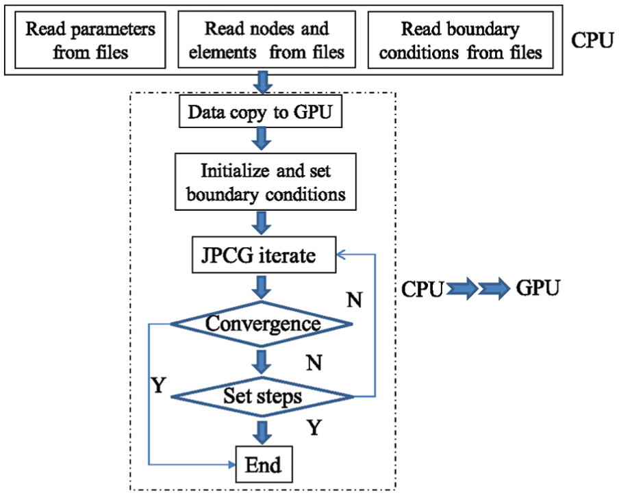
Flow chart of LSFEM.

As far as the GPU developed by NVIDIA is concerned, the latest GPU can support up to 1536 active threads per multiprocessor, which leads to more than 24,000 concurrently active threads per GPU if the device owns 16 multiprocessors. To fully exploit the parallelism of GPU, the kernels, for example, the functions or subroutines executed by GPU, regarding JPCG are carefully designed in terms of the organization of concurrent threads as well as the memory access hierarchy. Considering the limited resources offered by the GPU, including the count of registers and the amount of shared memory of each multiprocessor, a trade-off between the size of the thread-block and the occupancy of the GPU has to be made properly. Meanwhile, the concurrent threads running on GPU are organized and scheduled in wraps with 32 threads each. As a consequence, the number of threads contained in each thread-block is specified as 256 after counting the amount of the used resources in each kernel.

As aforementioned, most of the variables were stored in the device memory, called global memory in CUDA, due to the extremely limited amount of shared memory per multiprocessor. Compared with shared memory, the latency of accessing device memory is huge therefore unacceptable, ranging from 400 to 600 clock cycles per access. However, the latency can be hidden or reduced to the best degree by employing coalesced access technique wherein the device memory reads or stores by threads within a warp are coalesced into as few as one transaction. In order to achieve coalesced access, all variables stored in device memory are allocated with the dedicated function cudaMallocPitch.

General design of kernels

As the power of GPUs steadily increase, several GPU-boosted programs fail to achieve optimal parallel performance because they lack parallel scalability over the capacity of the underlying GPUs. Therefore, applications targeting on making full use of GPUs should expose as much parallelism as possible and efficiently map the parallelism onto GPUs so as to keep the hardware busy most of time. In order to realize full efficiency of GPUs, there are several approaches such as parallel execution between CPUs and GPUs using asynchronous functions, concurrent data transfer and execution, concurrent kernel executions by employing multiple execution mechanism and reducing divergence within kernels. From the perspective of kernel execution, the occupancy of GPU is not only determined by the number of thread-block, but also related to the size of grid (e.g. the number of thread-blocks) since multiple concurrent thread-blocks can reside on a multiprocessor for executing. Considering the characteristics of kernels implemented in this article, wherein the most significant performance limiter is the remarkable access latency due to the large amount of data allocated in device memory, we decided to improve the parallel performance by creating as much more thread-blocks as possible to hide the access latency, which is also the prerequisite for coalesced access as discussed above. Specially speaking, variables defined in the program, R , U and D for instance, either 2D or three-dimensional (3D), are all represented as vectors (one-dimensional (1D) matrix). Assuming that the kernel kerFunction is responsible for processing variable V and the length of V is SIZE_OF_V, then the size of grid for launching kernel kerFunction is determined by equation (16) since the size of thread-block is set equal to 256 as aforementioned

$$\mathrm{GRID}\mathrm{\_}\mathrm{SIZE}=\mathrm{SIZE}\mathrm{\_}\mathrm{OF}\mathrm{\_}\mathrm{V}/256$$

(16)

If the value of GRID_SIZE is greater than the number of the first dimension (x-dimension) of the maximum grid size retrieved by the CUDA runtime (API function cudaGetDeviceProperties), GRID_SIZE is then expressed as a 2D even a 3D matrix. Let dimGrid of type dim3 defined in CUDA be the grid size for launching kernel kerFunction, then we have

$$\mathrm{dimGrid}.\mathrm{x}\times \mathrm{dimGrid}.\mathrm{y}\times \mathrm{dimGrid}.\mathrm{z}=\mathrm{GRID}\_\mathrm{SIZE}$$

(17)

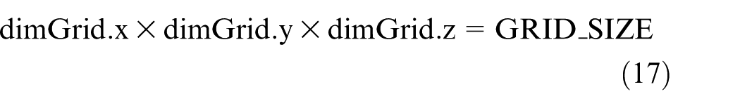
The latest GPU invented by NVIDIA support launching kernels with maximum grid size up to (2147483647, 65535, 65535), which is capable for kernel invocations in the majority of applications. However, an iteration procedure is employed if GRID_SIZE is even greater than the maximum size of a grid size.

Parallelization of matrix multiplication

In order to take full advantage of GPU’s computing capacity, the most time-consuming part should be found. In our CPU code of LSFEM, the JPCG part takes almost all the time. Kmly function, as in section ‘Least squares finite element method’, is part of JPCG. It is very suitable for parallel computing because matrix multiplication is carried out in each element. The JPCG code would be transformed to the form of kernel functions. Meanwhile, GPU runs kernel functions in the form of thread, which avoids branch statement and judgement statement. In consideration of that, the judgement statement of grid patterns in the Kmly functions is split into different kernel functions. In this way, judgement statement is avoided. Besides, in that way, grid pattern is determined before calculation, computation space requirement of shape functions is known, which avoids overmuch variables. This is beneficial for GPU, which has few registers. Besides, as each thread runs the same code, inner loop is transformed into common statement, which improves calculation efficiency.

Kernel functions of different grids are shown in Table 1.

Table 1.

The kernel function of different grids.

Kernel functions	Dimension	Rank	Linearization method
kernel_1orderQuadSimple2D	2D	First order	Simple
kernel_1orderQuadNewton2D	2D	First order	Newton
kernel_2orderQuadSimple2D	2D	Second order	Simple
kernel_2orderQuadNewton2D	2D	Second order	Newton
kernel_1orderQuadSimple3D	3D	First order	Simple
kernel_1orderQuadNewton3D	3D	First order	Newton
kernel_2orderQuadSimple3D	3D	Second order	Simple
kernel_2orderQuadNewton3D	3D	Second order	Newton

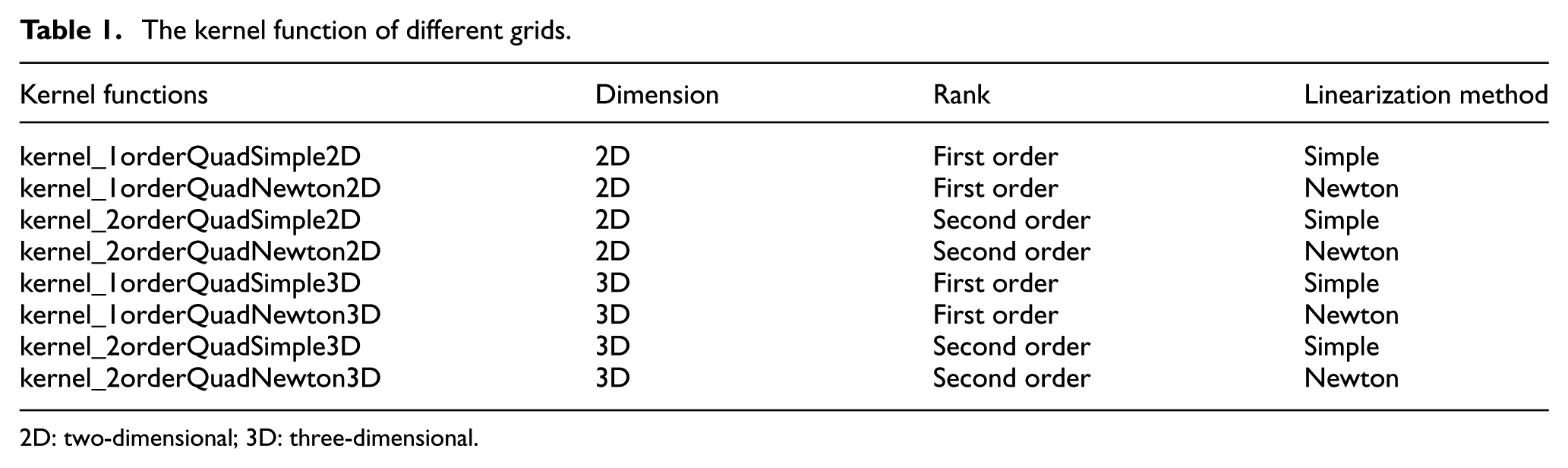
2D: two-dimensional; 3D: three-dimensional.

In addition to kernel functions, variable used in calculation should be transferred to GPU from CPU. Global variables used in CPU should be transferred into ones that can be used by GPU, which is realized by the introduction of pointer. Intermediate variable during calculation would be stored in the register, but array data could only be stored in local memory, which would slow down the calculation. In summary, usage of intermediate variable should be considered carefully.

GPU runs codes in high degree of parallelization. Only codes in same block are run in sequence. So it makes sense only in the range of same block. In GPU codes, when each thread in the same block reads data from the first node in an element, and nodes in one element are ordered anticlockwise, each thread would not interrupt each other, which has little influence on atomic operation. So in our case, nodes and elements are ordered to improve the efficiency of GPU parallel calculation.

Parallelization of JPCG loop

After transferring Kmly functions into kernel functions, the speed of calculation would be improved. However, other parts of JPCG loop are still computing serially. Also, there would be a lot of data exchange between CPU and GPU, which has a significant effect on efficiency. So, JPCG loop would be transferred into kernel functions.

In the transferring, it is noticed that JPCG loop is not a single parallel calculation, which makes it unsuitable for one kernel function. Each statement in the JPCG loop is transferred into one kernel function. There, JPCG loop would be carried out only in GPU, eliminating the need of data exchange between CPU and GPU, which improves efficiency.

One thing to be mentioned, for there is simple operation as dot product calculation in JPCG loop, it needs to consider whether it is worthwhile to transfer each statement into kernel function. There are two reasons for the answer yes. First, as each statement is carried out on GPU and data are stored on GPU, there is no need for data exchange between CPU and GPU during calculation. Second, GPU is designated for parallel computing and would optimize the calculation when carrying out kernel function in sequence, thus improving efficiency.

GPU has CUDA Basic Linear Algebra Subprograms (cuBLAS), which does matrix calculation in high efficiency. So they are used in this program. However, there are three statements that are not in the library. They are reciprocal calculation, matrix multiplication and boundary condition modification, which would be rewritten as follows:

• //kernel function for reciprocal calculation

• __global__ void gpuVecInvKernel ( unsigned int size, REAL * x)

• {

•  // Thread index

•  const unsigned int index = blockDim.x*blockIdx.x + threadIdx.x;

•  if ( index < size )

•  x[index] = 1.0 / x[index];

• }

• // kernel function for matrix multiplication

• __global__ void gpuVecVecMulKernel ( unsigned int size,

•      REAL * x, REAL * y, REAL * r )

• {

•  // Thread index

•  const unsigned int index = blockDim.x*blockIdx.x + threadIdx.x ;

•  if ( index < size )

•    r[index] = x[index]*y[index] ;

• }

• // kernel function for boundary condition modification

• __global__ void gpuBoundarySetKernel ( unsigned int size,

•      int *bcSet, REAL * bcVal, REAL * x )

• {

•  // Thread index

•  const unsigned int index = blockDim.x*blockIdx.x + threadIdx.x;

•  if ( index < size )

•    if (bcSet[index])

•    x[index] = bcVal[index];

• }

Parallel computing on multi-GPUs

With the development of hardware, multi-GPU platform has appeared. It has become possible to use several GPUs for computation. Based on that, parallel computing on multi-GPUs is carried out in this article.

Variable allocation

The difference between single GPU and multi-GPUs is in the allocation of variables. The distribution should be in balance.

For the convenience of presentation, we use two GPUs as an example. As JPCG loop is calculated in each element, the first GPU does calculation of the first half of all the elements, the second does that of latter ones. Also, variables related to each node would be distributed into two halves.

In addition, GPU needs to be designated the number of blocks when running kernel functions, in the form of kernel_function<<<GRID_SIZE, THREAD_BLOCK_ SIZE>>>(). GRID_SIZE stands for the number of blocks in each grid, which is related to the amount of variables. So in the transfer from single GPU to multi-GPUs, variables allocated to each GPU are reduced, which leads to change in GRID_SIZE.

Data transfer

Element data and node data are assigned in different GPUs. In the calculation process, we encountered a case that the calculation of the GPU No. 1 requires the use of variables on the GPU No. 2, which means the data to be used by the GPU No. 1 should be updated after each iteration calculation. Therefore, redundant memory holding the overlapping areas at the boundaries is allocated in multi-GPUs so as to eliminate the data exchange within one iteration of JPCG. Meanwhile, it is necessary to add one step to copy the data of these overlapping areas to the GPU that needs to use the data after each iteration. Two parts of the sentence were added into the program. One is to determine whether a node data is used by other GPUs, and the other is copy of the eligible data to the corresponding GPU. It is realized that the data exchanges is an important problem in implementing parallel computing on multi-GPUs and the overheads of data exchanges between multi-GPUs maybe degenerate the computing performance. At present, we focus on the calculation of GPU itself, and are not effective to deal with the data exchanges between multi-GPUs. Improvement of acceleration ratios can be achieved by minimizing data exchange between multi-GPUs in the next step.

Modification of cuBLAS functions

CuBLAS functions are used in multi-GPUs code, which is same as in single GPU code. However, cuBLAS functions are synchronous, which means that in multi-GPUs case, the second GPU runs the code after the first one is done. This means no improvement in efficiency. So cuBLAS functions are replaced by cuBLAS_V2 functions, which are asynchronous. GPUs run at the same time to improve efficiency.

Results of GPU calculation

Calculation model and computer platform

With the code mentioned above, lid-driven cavity flow problem was calculated, both on CPU and GPU, to compare calculation efficiency. A series of experiments were conducted in a lid-driven cavity of square cross section for Reynolds numbers between 3200 and 10,000 and spanwise aspect ratios between 0.25:1 and 1:1, which can be referred to Prasad and Koseff. ¹⁸ The velocity experiment result of Reynolds number of 3200 and spanwise aspect ratios of 1:1 was used to validate the simulation results of CPU and GPU. A lid-driven cavity square cross section model was created, as shown in Figure 2(a). The three dimensions are 1 and three different numbers of cells with 30³, 60³ and 120³ were created to assess the acceleration ratio. The boundary condition is that, the upper lid given driving velocity of 1 m/s, the rest set as wall. A steady solution was obtained with second-order spatial discretization schemes. Residuals were controlled under four orders of magnitude by 4000 outer loops and 200 inter loops.

Figure 2.

Calculation model and K20c: (a) lid-driven cavity model and (b) K20c.

NVIDIA Tesla K20c as GPU was used in this calculation, as shown in Figure 2(b). It has 2496 cores. It has a computing frequency of 700 MHz and a memory of 4 GB. CUDA 5.5 is supported. Two GPUs are used in multi-GPUs case. To compare with GPU, Intel E5-2697 V2 is used for CPU results, which has 12 cores with 24 threads, computing frequency of 2.6 GHz.

Accuracy and acceleration ratio

To validate the accuracy of single precision GPU code, lid-driven cavity flow was calculated both on CPU and GPU platforms. Result comparisons are shown in Figure 3. The agreement of dimensionless mean velocity between CPU result and test result indicates the code is correct. CPU and GPU get nearly the same velocity contour and the vorticity location. It should be pointed out that fewer particles are released in the post-processing lead to less pathlines in CPU result. If the same particles were released, the pathlines of them are consistent. Due to the few differences, we can believe the results of single GPU and dual GPUs codes are correct.

Figure 3.

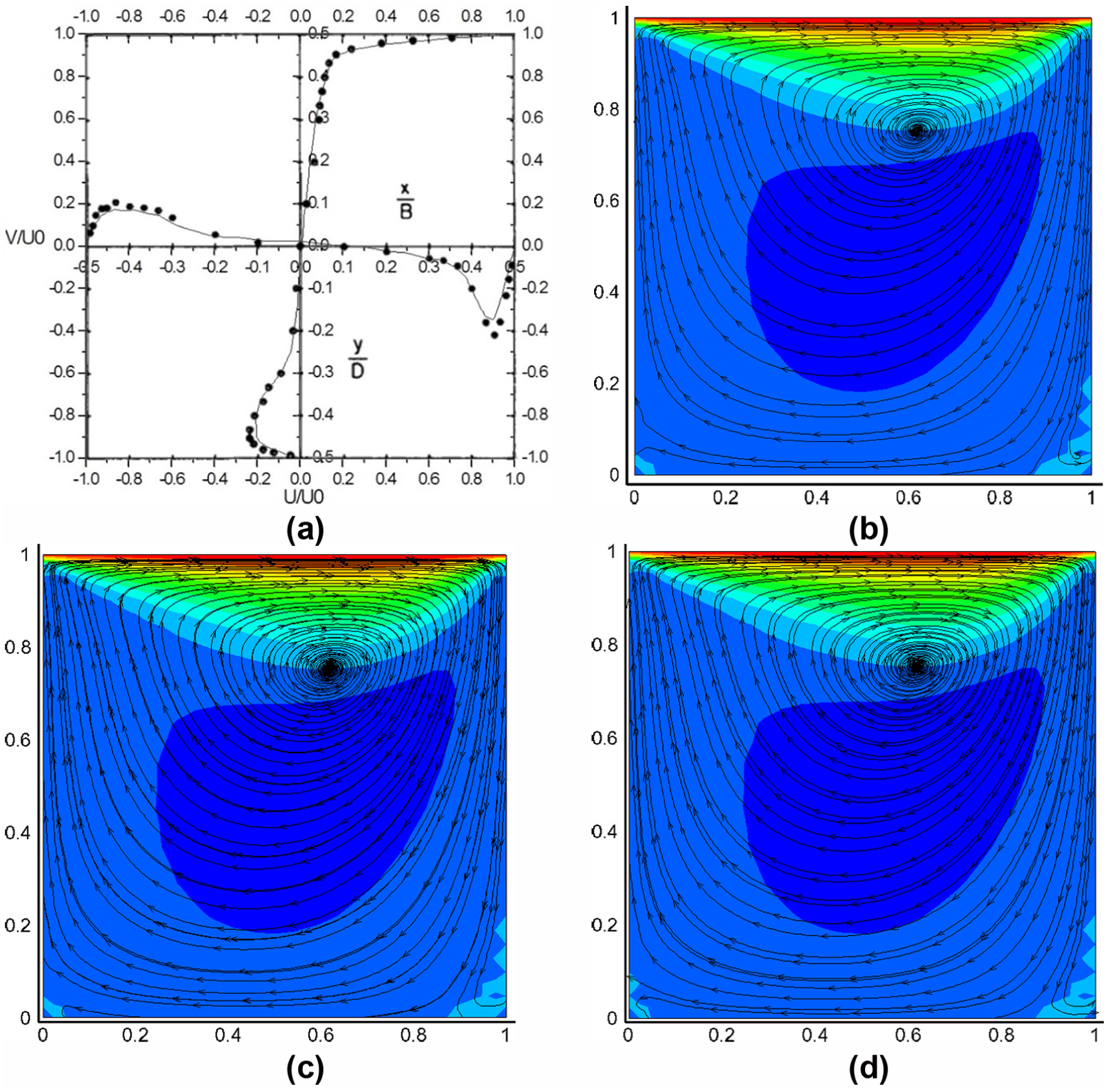
Result comparison in symmetric surface: (a) dimensionless mean velocity of CPU result and test result, (b) pathline and velocity contour of CPU result, (c) pathline and velocity contour of single GPU result and (d) pathline and velocity contour of two GPUs result.

Afterwards, lid-driven cavity flow cases with element number of 30³, 60³ and 120³ were calculated to assess the acceleration ratio. Companion between CPU and single GPU is shown in Table 2. It shows that the acceleration ratio is over 50 times in each case. This is a remarkable increase comparing with 7.7 times in Ding et al. ⁸ Therefore, LSFEM achieved a remarkable performance with GPU’s parallel computing ability. Besides, with the increase in element number, the acceleration ratio increases simultaneously, to a peak of 70.5.

Table 2.

Computational time and acceleration ratio between CPU (single core) and single GPU.

Case	Element number	CPU (s/10 steps)	GPU (s/10 steps)	Acceleration ratio
Cavity-30	303	414.3	7.4	56.0
Cavity-60	603	3239.9	49.1	66.0
Cavity-120	1203	26092.8	370.1	70.5

CPU: central processing unit; GPU: graphic processing unit.

Companion between CPU and dual GPUs is shown in Table 3. As calculation is separated into dual GPUs, the computing time can be seen as follows: time when only GPU No. 1 is calculating, time when dual GPUs are both calculating, time when only GPU No. 2 is calculating and time when dual GPUs are exchanging data. Obviously, the less the time when dual GPUs are exchanging data, the higher the acceleration ratio. When the element number is small (less than 60³), dual GPUs take more time than single GPU because of the time it takes to exchange data between GPUs. With the increase in element number, the proportion of time for data exchange decreases. The acceleration ratio of dual GPUs increases to 95.2, which is much higher than the case of single GPU. Multi-GPUs are more suitable for large-scale computing.

Table 3.

Computational time and acceleration ratio between CPU (single core) and dual GPUs.

Case	Element number	CPU (s/10 steps)	1 GPU (s/10 steps)	2 GPUs (s/10 steps)	Acceleration ratio
Cavity-30	303	414.3	7.4	11.1	37.3
Cavity-60	603	3239.9	49.1	65.9	49.2
Cavity-120	1203	26092.8	370.1	274.1	95.2

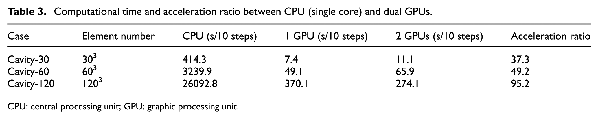
CPU: central processing unit; GPU: graphic processing unit.

Conclusion

In this article, parallel computing based on LSFEM was carried out on GPU. It is pointed out that JPCG is the most time-consuming part. The modification of branch statement and kernel function was done and calculation on single GPU was realized. Results of lid-driven cavity flow show the accuracy of GPU calculation. A speedup ratio of 70.5 times is reached in the case of element number 120³, which is remarkable in saving computational time.

Variable allocation, data transfer and modification of cuBLAS functions were done on multi-GPUs platform. An acceleration ratio of 49.2 times was reached in the case of small element number 60³, slower than single GPU. With the increase in the element number, acceleration ratio of 95.2 times was reached when element number increases to 120³, much faster than single GPU.

In addition, acceleration ratio of GPUs increases with the increase in element number, especially in the case of multi-GPUs. The code in our article is suitable for more than dual GPUs. Calculation and optimization on more GPUs will be done to get higher acceleration ratio.