Sage Journals: Discover world-class research

Abstract

With the aim of dynamic modeling of the SCARA robot subjected to space trajectory constraint to satisfy repetitive tasks with higher accuracy, a succinct and explicit equation of motion based on Udwadia–Kalaba theory is established. The trajectory constraint, which is regarded as the external constraints imposed on the system, is integrated into the dynamic modeling of the system dexterously. The explicit expression of constraint torques required to satisfy constraints and explicit dynamic equation of the system without Lagrange multiplier are obtained. However, constraint violation arises when the initial conditions are incompatible with the constraint equations. Baumgarte stabilization method is considered for constraint violation suppression. Simulations of the varying law of the generalized coordinate variables and the trajectories of the SCARA robot are performed to demonstrate the simplicity and accuracy of the method.

Keywords

SCARA robot constraint dynamic modeling Udwadia–Kalaba theory Baumgarte stabilization method

Introduction

As a nonlinear dynamic system, the SCARA robot with four joints (e.g. three revolute and one prismatic) has better repeatability of robot movements and higher accuracy in their performance. The SCARA robot is required to follow the desired trajectory for many applications during the current stage of industrial development for productivity enhancement and quality improvement in manufactured products, such as pick and place, assembly, and packaging.

In fact, dynamic modeling of the SCARA robot to realize the desired trajectory is within the dynamic modeling of constrained multibody system. One of the key issues to address in multibody dynamics is to obtain explicit equations of motion for constrained dynamical systems.¹ Constrained dynamical systems are conventional model based on Lagrangian formulation in which Lagrangian multiplier is determined relied on problem-specific approaches.² When the number of the constraint equations is not equal to the number of generalized variables, the traditional Lagrangian formulation is invalidated. Moreover, there are many alternative approaches available to model constrained dynamical systems, which also need auxiliary variables. For example, Hamel’s equations require Quasi Velocity as auxiliary term; Kane’s³ equations require a set of Pseudo-Generalized Speed as auxiliary terms; Gibbs–Appell formulation requires Pseudo-Velocity and Pseudo-Acceleration as auxiliary terms;⁴ and Poincaré equations require a set of Pseudo-Velocity as auxiliary terms. It is worth noting that only the numerical solutions can be obtained by all of the aforementioned methods.

An explicit equation of motion for constrained systems, called the Udwadia–Kalaba equation, was proposed by Firdaus E. Udwadia and Robert E. Kalaba⁵ in 1992, which opens up a new way of modeling complex multibody systems. This method provides a general structure for the explicit equations of motion for mechanical systems subjected to holonomic and nonholonomic equality constraints.^6,7 Moreover, it is not an issue for Udwadia–Kalaba equation based on the Gauss’ principle of least constraint, and the optimal value of the generalized variables solution can still be obtained by the Moore–Penrose generalized inverse when the number of the constraint equations is not equal to the number of generalized variables. Udwadia and colleagues^8–11 also effectively dealt with the dynamics and control of nonlinear uncertain systems to benefit the basic research and further application of this method. It has been studied in some application fields, such as industrial robot,¹² parallel robot,¹³ flexible multibody systems,¹⁴ railway vehicles collision,¹⁵ machine fish,¹ control of tethered satellites,¹⁶ rigid multibody systems,¹⁷ and mobile robots.¹⁸

Like many other robots, the SCARA robot is often required to achieve some specified space trajectories (i.e. trajectory constraint). Only a few scholars focus on the explicit dynamical equations for the SCARA robot subjected to constraints. In this article, a succinct and explicit equation of motion based on the Udwadia–Kalaba theory for the SCARA robot is established. However, constraint violation arises when the initial conditions are incompatible with the constraint equations. Due to the simplicity and easiness for computational implementation, Baumgarte stabilization method, proposed by Baumgarte¹⁹ and then developed in numerous contributions, is probably the most popular and attractive technique to implement the control of constraint violation.²⁰ Therefore, Baumgarte stabilization method is considered for constraint violation suppression. The comparison of simulation results of the dynamic modeling shows that the derived equations can successfully address the dynamic modeling for the SCARA robot subjected to trajectory constraints to satisfy repetitive tasks with higher accuracy. Finally, conclusions of this work and future tasks are given.

Udwadia–Kalaba theory

The explicit equation of motion for a constrained dynamical system proposed by Udwadia and Kalaba⁵ is derived in this section using a systematic general three-step procedure: (1) consideration of the so-called unconstrained system of equations obtained using Newtonian or Lagrangian mechanics, (2) description of the constraints required to model the given constrained system, and (3) expression of the constraint torques for system to satisfy the given constraints.

Unconstrained multibody dynamics

Considering an unconstrained multibody system characterized by n generalized coordinates $q : = [q_{1} q_{2} \dots q_{n}]^{T} \in R^{n}$ , the dynamics of the system is described as

M (q, t) \overset{\cdot\cdot}{q} = Q (q, \dot{q}, t)

(1)

in which $M (q, t) \in R^{n \times n}$ denotes a symmetric positive-definite mass matrix of the system related to $q$ , t; $Q (q, \overset{\cdot}{q}, t) \in R^{n}$ collects the normal and Coriolis inertial terms and the applied forces related to $q$ , $\overset{\cdot}{q}$ , t; $q \in R^{n}$ is the generalized coordinate n-vector; $\overset{\cdot}{q} \in R^{n}$ is the generalized velocity; and $\overset{\cdot\cdot}{q} \in R^{n}$ is the generalized acceleration.

The generalized acceleration of the unconstrained dynamical system, defined as $a (q, \overset{\cdot}{q}, t)$ , is of the form

a (q, \dot{q}, t) : = M^{- 1} (q, t) Q (q, \dot{q}, t)

(2)

Constraint description

It is assumed that the system is subjected to p sufficiently smooth control requirements as constraints, which include all the usual varieties of holonomic and/or nonholonomic constraints and can be describes as⁹

φ_{i} (q, \dot{q}, t) = 0, i = 1, 2, \dots, p

(3)

Equation (3) can be simplified as

Φ = [φ_{1} φ_{2} \dots φ_{p}]^{T} = 0

(4)

Differentiating the usual constraint equation (4) with respect to time t once (for nonholonomic constraints) or twice (for holonomic constraints) yields a set of constraint equations in matrix form as⁹

A (q, \overset{\cdot}{q}, t) \overset{\cdot\cdot}{q} = b (q, \overset{\cdot}{q}, t)

(5)

in which $A (q, \overset{\cdot}{q}, t) \in R^{p \times n}$ denotes the constraint matrix, and $b (q, \overset{\cdot}{q}, t) \in R^{p}$ is a p-vector.

Constrained multibody dynamics

The intent needs to establish the explicit equations of motion with constraints. Additional generalized forces of constraints arise due to the presence of constraints. Accordingly, the actual explicit equation of motion of the constrained system can be assumed to take the form

M (q, t) \overset{\cdot\cdot}{q} = Q (q, \overset{\cdot}{q}, t) + Q^{c} (q, \overset{\cdot}{q}, t)

(6)

in which $Q^{c} (q, \overset{\cdot}{q}, t) \in R^{n}$ is the constraint forces imposed on the system.

Obtaining the constraint torques is a main goal in the modeling of constrained dynamical system. Udwadia and Kalaba⁷ proposed that the constraint torque vector is explicitly given by

Q^{c} = M^{1 / 2} B^{+} (b - A M^{- 1} Q)

(7)

in which $B (q, t) : = A (q, \overset{\cdot}{q}, t) M^{- 1 / 2} (q, t)$ , and the superscript “+” denotes the Moore–Penrose generalized inverse.

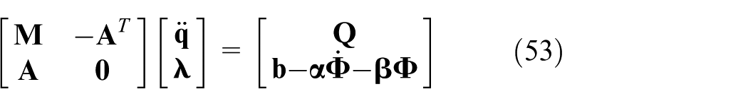
The explicit dynamical equation of the constrained system called as the Udwadia–Kalaba theory is denoted in the following general form^5,9

M \overset{\cdot\cdot}{q} = Q + M^{- 1 / 2} B^{+} (b - A M^{- 1} Q)

(8)

Premultiplying both sides of equation (8) with $M^{- 1}$ , the acceleration of the constrained system can be obtained

\overset{\cdot\cdot}{q} = M^{- 1} Q + M^{- 1 / 2} B^{+} (b - B M^{- 1 / 2} Q)

(9)

The standard Lagrange multiplier formulation of the constrained dynamics is in the following form

[\begin{matrix} M & - A^{T} \\ A & 0 \end{matrix}] [\begin{matrix} \overset{\cdot\cdot}{q} \\ λ \end{matrix}] = [\begin{matrix} Q \\ b \end{matrix}]

(10)

in which Lagrange multiplier $λ = (A M^{- 1} A^{T})^{- 1} (b - A M^{- 1} Q)$ .

Dynamic modeling of SCARA robot

Consider the SCARA robot illustrated in Figure 1. The generalized coordinates of the system are denoted as $q = [q_{1} q_{2} q_{3} q_{4}]^{T}$ .

Figure 1.

Sketch map of the SCARA robot manipulator subject to constraint.

Unconstrained dynamics

Result

The equations of motion of the unconstrained dynamical system are established first using the traditional Lagrange method

τ = M (q) \cdot \overset{\cdot\cdot}{q} + C \cdot \overset{\cdot}{q} + G (q)

(11)

in which $M (q) \in R^{4 \times 4}$ is the mass matrix; $C \cdot \overset{\cdot}{q} \in R^{4 \times 1}$ is the centrifugal force and Coriolis force matrix; $G (q) \in R^{4 \times 1}$ is the gravitational force; $q, \overset{\cdot}{q}, \overset{\cdot\cdot}{q} \in R^{4 \times 1}$ are the generalized position, velocity, and acceleration, respectively; $τ \in R^{4 \times 1}$ is the joint torque vector; and²¹

M_{ij} (q) = \sum_{l = max (i, j)}^{n} ξ_{i}^{T} A_{li}^{T} M'_{l} A_{lj} ξ_{j}

(12)

C_{ij} (q) = \frac{1}{2} \sum_{k = 1}^{n} (\frac{\partial M_{ij}}{\partial q_{k}} + \frac{\partial M_{ik}}{\partial q_{j}} - \frac{\partial M_{kj}}{\partial q_{i}}) {\overset{\cdot}{q}}_{k}

(13)

G (\overset{\cdot}{q}, q) = \frac{\partial V}{\partial q}

(14)

Proof

The coordinate frame relative to the base frame of the robot is represented as

g_{S C_{i}} (q) = e^{{\hat{ξ}}_{1} q_{1}} \dots e^{{\hat{ξ}}_{i} q_{i}} g_{S C_{i}} (0)

(15)

in which $C_{i}$ is attached to the mass center of the ith link of the SCARA robot; $S$ is the base frame of the robot; $g_{S C_{i}} (q) = (R_{S C_{i}}, t_{S C_{i}}) \in SE (3)$ is the transformation between $C_{i}$ and $S$ , and $g_{S C_{i}} (0)$ is the transformation between $C_{i}$ and $S$ at $q = 0$ ; ${\hat{ξ}}_{i}$ is referred to a skew-symmetric matrix. For the revolute joint, the joint twists $ξ_{i}$ is expressed as $ξ_{i} = [\begin{matrix} - ω_{i} \times L_{i} \\ ω_{i} \end{matrix}]$ , in which $ω_{i} \in R^{3}$ is a unit vector which specifies the direction of rotation; $L_{i} \in R^{3}$ is any point on the axis; for the prismatic joint, the twist $ξ_{i}$ is expressed as $ξ_{i} = [\begin{matrix} v_{i} \\ 0 \end{matrix}]$ , in which $v_{i} \in R^{3}$ is a unit vector in the direction of translation.

The body velocity of the mass center of the ith link is described as

V_{S C_{i}}^{b} = J (q) \overset{\cdot}{q}

(16)

in which $J (q)$ is the body Jacobian corresponding to $g_{S C_{i}} (q)$ , and

J (q) = [\begin{matrix} ξ_{1}^{†} & \dots & ξ_{i}^{†} & 0 & \dots & 0 \end{matrix}]

(17)

in which $ξ_{j}^{†} = {Ad}_{(e^{{\hat{ξ}}_{j} q_{j}} \dots e^{{\hat{ξ}}_{i} q_{i}} g_{S C_{i}} (0))}^{- 1} ξ_{j} \begin{matrix} (j \leq i) \end{matrix}$ is the jth instantaneous joint twist relative to the ith link frame $C_{i}$ .

The total kinetic energy of the robot has the form

\begin{matrix} T (\overset{\cdot}{q}, q) = \sum_{i = 1}^{n} T_{i} (\overset{\cdot}{q}, q) = \sum_{i = 1}^{n} \frac{1}{2} {(V_{S C_{i}}^{b})}^{T} M_{i} V_{S C_{i}}^{b} \\ = \sum_{i = 1}^{n} \frac{1}{2} {\overset{\cdot}{q}}^{T} J_{i}^{T} (q) M_{i} J_{i} (q) \overset{\cdot}{q} = : \frac{1}{2} {\overset{\cdot}{q}}^{T} M (q) \overset{\cdot}{q} \end{matrix}

(18)

in which $T_{i} (\overset{\cdot}{q}, q)$ and $M_{i}$ are the kinetic energy and the generalized inertia matrix of the ith link, respectively.

The total potential energy has the form

V (q) = \sum_{i = 1}^{n} V_{i} (q) = \sum_{i = 1}^{n} m_{i} g h_{i} (q)

(19)

in which $V_{i} (q)$ is the potential energy of the ith link; $m_{i}$ is the mass of the ith link; $g$ is the gravitational constant; and $h_{i} (q)$ is the height of the mass center of the ith link.

The Lagrange function can be obtained as

\begin{matrix} L (\overset{\cdot}{q}, q) = \sum_{i = 1}^{n} (T_{i} (\overset{\cdot}{q}, q) - V_{i} (q)) \\ = \frac{1}{2} {\overset{\cdot}{q}}^{T} M (q) \overset{\cdot}{q} - V (q) = \frac{1}{2} \sum_{i, j = 1}^{n} M_{ij} (q) {\overset{\cdot}{q}}_{i} {\overset{\cdot}{q}}_{j} - V (q) \end{matrix}

(20)

So far, the equations of motion can be obtained by substituting into Lagrange’s equations

\frac{d}{d t} \frac{\partial L}{\partial {\overset{\cdot}{q}}_{i}} - \frac{\partial L}{\partial q_{i}} = F_{i}

(21)

in which $F_{i}$ represents the generalized forces acting on the ith joint, and

\frac{d}{d t} \frac{\partial L}{\partial {\overset{\cdot}{q}}_{i}} = \frac{d}{d t} (\sum_{j = 1}^{n} M_{ij} {\overset{\cdot}{q}}_{j}) = \sum_{j = 1}^{n} (M_{ij} {\overset{\cdot\cdot}{q}}_{j} + {\overset{\cdot}{M}}_{ij} {\overset{\cdot}{q}}_{j})

(22)

\frac{\partial L}{\partial q_{i}} = \frac{1}{2} \sum_{j, k = 1}^{n} \frac{\partial M_{kj}}{\partial q_{i}} {\overset{\cdot}{q}}_{k} {\overset{\cdot}{q}}_{j} - \frac{\partial V}{\partial q_{i}}

(23)

1. The matrix $M (q) \in R^{n \times n}$ is obtained using the following procedure.

In terms of the link Jacobians, $J_{i}$ , the manipulator inertia matrix is defined as

M (q) = \sum_{i = 1}^{n} J_{i}^{T} (q) M_{i} J_{i} (q)

(24)

in which $J_{i} (q) = A d_{g_{S C_{i} (0)}^{- 1}} [\begin{matrix} A_{i 1} ξ_{1} & \dots & A_{ii} ξ_{i} 0 & \dots & 0 \end{matrix}]$ . $A d_{g_{S C_{i} (0)}^{- 1}}$ is referred to as the adjoint transformation associated with $g_{S C_{i} (0)}^{- 1}$ . $A d_{g_{S C_{i}}^{- 1}} A_{ij} ξ_{j}$ represents the jth column of the body Jacobian for the ith link, in which $A_{ij}$ is the adjoint transformation given by

A_{ij} = {\begin{matrix} {Ad}_{(e^{{\hat{ξ}}_{j + 1} q_{j + 1}} \dots e^{{\hat{ξ}}_{i} q_{i}})}^{- 1} \begin{matrix} i \end{matrix} > j \\ I i = j \\ 0 i < j \end{matrix}

(25)

The inertia of the ith link reflected into the base frame of the manipulator, $M'_{i}$ , is given by

M'_{i} = {Ad}_{g_{S C_{i} (0)}^{- 1}}^{T} M_{i} A d_{g_{S C_{i} (0)}^{- 1}}

(26)

Using the notation defined above, the inertia matrix for the manipulator can be obtained as²¹

M_{ij} (q) = \sum_{l = max (i, j)}^{n} ξ_{i}^{T} A_{li}^{T} M'_{l} A_{lj} ξ_{j}

(27)

2. Substituting equations (22) and (23) into equation (21) and expanding ${\overset{\cdot}{M}}_{ij}$ in terms of partial derivatives, one can obtain

\begin{matrix} \sum_{j = 1}^{n} M_{ij} (q) {\overset{\cdot\cdot}{q}}_{j} + \sum_{j, k = 1}^{n} (\frac{\partial M_{ij}}{\partial q_{k}} {\overset{\cdot}{q}}_{j} {\overset{\cdot}{q}}_{k} - \frac{1}{2} \frac{\partial M_{kj}}{\partial q_{i}} {\overset{\cdot}{q}}_{k} {\overset{\cdot}{q}}_{j}) \\ + \frac{\partial V}{\partial q_{i}} (q) = F_{i}, i = 1, 2, \dots, n \end{matrix}

(28)

Rearranging all the terms, equation (28) can be rewritten as

\begin{matrix} \sum_{j = 1}^{n} M_{ij} (q) {\overset{\cdot\cdot}{q}}_{j} + \sum_{j, k = 1}^{n} Γ_{ijk} {\overset{\cdot}{q}}_{j} {\overset{\cdot}{q}}_{k} + \frac{\partial V}{\partial q_{i}} (q) = F_{i}, \\ i = 1, 2, \dots, n \end{matrix}

(29)

in which $Γ_{ijk} = \frac{1}{2} (\frac{\partial M_{ij} (q)}{\partial q_{k}} + \frac{\partial M_{ik} (q)}{\partial q_{j}} - \frac{\partial M_{kj} (q)}{\partial q_{i}})$ .

The matrix $C (\overset{\cdot}{q}, q)$ is considered to be defined in order to put equation (29) back into vector form²¹

C_{ij} (\overset{\cdot}{q}, q) = \sum_{k = 1}^{n} Γ_{ijk} {\overset{\cdot}{q}}_{K} = \frac{1}{2} \sum_{k = 1}^{n} (\frac{\partial M_{ij}}{\partial q_{k}} + \frac{\partial M_{ik}}{\partial q_{j}} - \frac{\partial M_{kj}}{\partial q_{i}}) {\overset{\cdot}{q}}_{k}

(30)

in which $\frac{\partial M_{i j}}{\partial q_{k}} = \sum_{l = \max (i, j)}^{n} ({[A_{k i} ξ_{i}, ξ_{k}]}^{T} A_{l k}^{T} {M'}_{l} A_{l j} ξ_{j} + ξ_{i}^{T} A_{l i}^{T} {M'}_{l} A_{l k} [A_{k j} ξ_{j}, ξ_{k}])$ .

3. Finally, the gravitational forces on the manipulator are written as²¹

G (\overset{\cdot}{q}, q) = \frac{\partial V}{\partial q}

(31)

For the SCARA robot, considering $g_{ST} = (R_{ST}, t_{ST}) \in SE (3)$ , the transformation between tool and base frames at $q = 0$ is given by

g_{ST} (0) = [\begin{matrix} I & (\begin{matrix} 0 \\ l_{1} + l_{2} \\ l_{0} \end{matrix}) \\ 0 & 1 \end{matrix}]

(32)

For the three revolute joints, the direction of rotation is described as $ω_{1} = ω_{2} = ω_{3} = [\begin{matrix} 0 & 0 & 1 \end{matrix}]^{T}$ , and the points on the axis are described as $L_{1} = [\begin{matrix} 0 & 0 & 1 \end{matrix}]^{T}$ , $L_{2} = [\begin{matrix} 0 & l_{1} & 0 \end{matrix}]^{T}$ , and $L_{3} = [\begin{matrix} 0 & l_{1} + l_{2} & 0 \end{matrix}]^{T}$ . For the prismatic joint, the direction of translation is described as $v_{4} = [\begin{matrix} 0 & 0 & 1 \end{matrix}]$ . This yields twists

\begin{matrix} ξ_{1} = {[\begin{matrix} 0 & 0 & 0 & 0 & 0 & 1 \end{matrix}]}^{T} \\ ξ_{2} = {[\begin{matrix} l_{1} & 0 & 0 & 0 & 0 & 1 \end{matrix}]}^{T} \\ ξ_{3} = {[\begin{matrix} l_{1} + l_{2} & 0 & 0 & 0 & 0 & 1 \end{matrix}]}^{T} \\ ξ_{4} = {[\begin{matrix} 0 & 0 & 1 & 0 & 0 & 0 \end{matrix}]}^{T} \end{matrix}

(33)

The inertia matrix $M (q) \in R^{4 \times 4}$ for the SCARA robot can be derived as²¹

M (q) = [\begin{matrix} α + β + 2 γ c_{2} & β + γ c_{2} & δ & 0 \\ β + γ c_{2} & β & δ & 0 \\ δ & δ & δ & 0 \\ 0 & 0 & 0 & m_{4} \end{matrix}]

(34)

in which $α = I_{z 1} + r_{1}^{2} m_{1} + l_{1}^{2} m_{2} + l_{1}^{2} m_{3} + l_{1}^{2} m_{4}$ , $β = I_{z 2} + I_{z 3} + I_{z 4} + l_{2}^{2} m_{3} + l_{2}^{2} m_{4} + m_{2} r_{2}^{2}$ , $γ = l_{1} l_{2} m_{3} + l_{1} l_{2} m_{4} + l_{1} m_{2} r_{2}$ , and $δ = I_{z 3} + I_{z 4}$ . Note that $c_{i} = \cos q_{i}$ , $s_{i} = \sin q_{i}$ , $c_{ij} = \cos (q_{i} + q_{j})$ , and $s_{ij} = \sin (q_{i} + q_{j})$ .

The Coriolis matrix for the SCARA robot can be obtained as²¹

C (q, \overset{\cdot}{q}) = [\begin{matrix} - γ \sin q_{2} {\overset{\cdot}{q}}_{2} & - γ \sin q_{2} ({\overset{\cdot}{q}}_{1} + {\overset{\cdot}{q}}_{2}) & 0 & 0 \\ γ \sin q_{2} {\overset{\cdot}{q}}_{1} & 0 & 0 & 0 \\ 0 & 0 & 0 & 0 \\ 0 & 0 & 0 & 0 \end{matrix}]

(35)

The gravitational forces on the SCARA robot is expressed as²¹

G (q, \overset{\cdot}{q}) = {[\begin{matrix} 0 & 0 & 0 & m_{4} g \end{matrix}]}^{T}

(36)

Constraint description

The exponential of this twist is given by

e^{\hat{ξ} q} = [\begin{matrix} e^{\hat{ω} q} (I - e^{\hat{ω} q}) (ω \times v) + q ω ω^{T} v \\ 01 \end{matrix}]

(37)

in which

\begin{matrix} e^{\hat{ω} q} = I + \hat{ω} s q + {\hat{ω}}^{2} (1 - c q) \\ = [\begin{matrix} ω_{1}^{2} (1 - c q) + c q & ω_{1} ω_{2} (1 - c q) - ω_{3} s q & ω_{1} ω_{3} (1 - c q) + ω_{2} s q \\ ω_{1} ω_{2} (1 - c q) + ω_{3} s q & ω_{2}^{2} (1 - c q) + c q & ω_{2} ω_{3} (1 - c q) - ω_{1} s q \\ ω_{1} ω_{3} (1 - c q) - ω_{2} s q & ω_{2} ω_{3} (1 - c q) + ω_{1} s q & ω_{3}^{2} (1 - c q) + c q \end{matrix}] \\ c q = \cos q, s q = \sin q \end{matrix}

The forward kinematic map of the SCARA robot is given by

g_{ST} (q) = e^{{\hat{ξ}}_{1} q_{1}} e^{{\hat{ξ}}_{2} q_{2}} e^{{\hat{ξ}}_{3} q_{3}} e^{{\hat{ξ}}_{4} q_{4}} g_{ST} (0) = [\begin{matrix} R (q) & p (q) \\ 0 & 1 \end{matrix}]

(38)

in which the individual exponentials have the form

\begin{matrix} e^{{\hat{ξ}}_{1} q_{1}} = [\begin{matrix} c_{1} & - s_{1} & 0 & 0 \\ s_{1} & c_{1} & 0 & 0 \\ 0 & 0 & 1 & 0 \\ 0 & 0 & 0 & 1 \end{matrix}], \\ e^{{\hat{ξ}}_{2} q_{2}} = [\begin{matrix} c_{2} & - s_{2} & 0 & l_{1} s_{2} \\ s_{2} & c_{2} & 0 & l_{1} (1 - c_{2}) \\ 0 & 0 & 1 & 0 \\ 0 & 0 & 0 & 1 \end{matrix}] \\ e^{{\hat{ξ}}_{3} q_{3}} = [\begin{matrix} c_{3} & - s_{3} & 0 & (l_{1} + l_{2}) s_{3} \\ s_{3} & c_{3} & 0 & (l_{1} + l_{2}) (1 - c_{3}) \\ 0 & 0 & 1 & 0 \\ 0 & 0 & 0 & 1 \end{matrix}], \\ e^{{\hat{ξ}}_{4} q_{4}} = [\begin{matrix} 1 & 0 & 0 & 0 \\ 0 & 1 & 0 & 0 \\ 0 & 0 & 1 & q_{4} \\ 0 & 0 & 0 & 1 \end{matrix}] \end{matrix}

Expanding the terms in the product of exponentials formula yields

\begin{matrix} g_{ST} (q) = [\begin{matrix} R (q) & p (q) \\ 0 & 1 \end{matrix}] \\ = [\begin{matrix} c_{123} & - s_{123} & 0 & - l_{1} s_{1} - l_{2} s_{12} \\ s_{123} & c_{123} & 0 & l_{1} c_{1} + l_{2} c_{12} \\ 0 & 0 & 1 & l_{0} + q_{4} \\ 0 & 0 & 0 & 1 \end{matrix}] \end{matrix}

(39)

The end-effector of the SCARA robot moves along space trajectory to complete the given tasks. The desired space trajectory, which is regarded as constraints, is presented as follows.

The position constraints can be described as

\begin{matrix} x = 0.05 \sin (0.4 π t) \\ y = 0.35 + 0.05 \cos (0.4 π t) \\ z = 0.02 t \end{matrix}

(40)

The following elementary rotations about the x-, y-, and z-axis are defined as

\begin{matrix} R_{x} (θ) : e^{\hat{x} θ} = [\begin{matrix} 1 & 0 & 0 \\ 0 & \cos θ & - \sin θ \\ 0 & \sin θ & \cos θ \end{matrix}] \\ R_{y} (θ) : e^{\hat{y} θ} = [\begin{matrix} \cos θ & 0 & \sin θ \\ 0 & 1 & 0 \\ - \sin θ & 0 & \cos θ \end{matrix}] \\ R_{z} (θ) : e^{\hat{z} θ} = [\begin{matrix} \cos θ & - \sin θ & 0 \\ \sin θ & \cos θ & 0 \\ 0 & 0 & 1 \end{matrix}] \end{matrix}

(41)

ZYZ Euler angles are used to express the orientation of the end-effector of the SCARA robot. The equivalent rotation matrix is denoted as

\begin{matrix} {{}_{T}^{S}R}_{zyz} (φ, ψ, γ) = R_{z} (φ) R_{y} (ψ) R_{z} (γ) = e^{\hat{z} φ} e^{\hat{y} ψ} e^{\hat{z} γ} \\ = [\begin{matrix} c φ c ψ c γ - s φ s γ & - c φ c ψ s γ - s φ c γ & c φ s ψ \\ s φ c ψ c γ + c φ s γ & - s φ c ψ s γ + c φ c γ & s φ s ψ \\ - s ψ c γ & s ψ s γ & c ψ \end{matrix}] \end{matrix}

(42)

Conversely, equivalent ZYZ Euler angles can be solved by the rotation matrix, as shown below. If

{}_{T}^{S}R = [\begin{matrix} r_{11} & r_{12} & r_{13} \\ r_{21} & r_{22} & r_{23} \\ r_{31} & r_{32} & r_{33} \end{matrix}] = [\begin{matrix} c_{124} & - s_{123} & 0 \\ s_{123} & c_{123} & 0 \\ 0 & 0 & 1 \end{matrix}]

(43)

and $\sin ψ \neq 0$ , then

\begin{matrix} φ = A \tan 2 (r_{23}, r_{13}) \\ ψ = A \tan 2 (\sqrt{r_{31}^{2} + r_{32}^{2}}, r_{33}) \\ γ = A \tan 2 (r_{32}, - r_{31}) \end{matrix}}

(44)

The solution of $ψ$ is always in the range of $0 \leq ψ \leq 180 \circ$ , although two solutions can be obtained from $\sin ψ = \sqrt{r_{31}^{2} + r_{32}^{2}}$ . The above solutions degenerate when $ψ = 0 \circ$ or $180 \circ$ ; at this point, only the sum or difference between $φ$ and $γ$ is obtained. $φ = 0 \circ$ is usually selected. If $ψ = 0 \circ$ , then

{\begin{matrix} α = 0 \circ \\ β = 0 \circ \\ γ = A \tan 2 (- r_{12}, r_{11}) \end{matrix}

(45)

The orientation constraint equation combined with equation (43) can be derived as

q_{1} + q_{2} + q_{3} = 0

(46)

Now that there are the following four constraints in total

{\begin{matrix} - l_{1} s_{1} - l_{2} s_{12} = 0.05 \sin (0.4 π t) \\ l_{1} c_{1} + l_{2} c_{12} = 0.35 + 0.05 \cos (0.4 π t) \\ q_{1} + q_{2} + q_{3} = 0 \\ q_{4} + l_{0} = 0.02 t \end{matrix}

(47)

In general, the constraint equations may be thought of as a set of p (p = 4) constraints of the form

\begin{matrix} Φ (t) = [\begin{matrix} φ_{1} \\ φ_{2} \\ φ_{3} \\ φ_{4} \end{matrix}] \\ = [\begin{matrix} - l_{1} s_{1} - l_{2} s_{12} - 0.05 \sin (0.4 π t) \\ l_{1} c_{1} + l_{2} c_{12} - 0.35 - 0.05 \cos (0.4 π t) \\ q_{1} + q_{2} + q_{3} \\ q_{4} + l_{0} - 0.02 t \end{matrix}] = 0 \end{matrix}

(48)

Differentiating equation (48) with respect to time t twice yields the second-order constraints

A \overset{\cdot\cdot}{q} = b

in which

\begin{matrix} A = [\begin{matrix} - l_{1} c_{1} - l_{2} c_{12} & - l_{2} c_{12} & 0 & 0 \\ - l_{1} s_{1} - l_{2} s_{12} & - l_{2} s_{12} & 0 & 0 \\ 1 & 1 & 1 & 0 \\ 0 & 0 & 0 & 1 \end{matrix}] \\ b = [\begin{matrix} - {\overset{\cdot}{q}}_{1}^{2} l_{1} s_{1} - {({\overset{\cdot}{q}}_{1} + {\overset{\cdot}{q}}_{2})}^{2} l_{2} s_{12} - 0.05 \times {(0.4 π)}^{2} \sin (0.4 π t) \\ {\overset{\cdot}{q}}_{1}^{2} l_{1} c_{1} + {({\overset{\cdot}{q}}_{1} + {\overset{\cdot}{q}}_{2})}^{2} l_{2} c_{12} - 0.05 \times {(0.4 π)}^{2} \cos (0.4 π t) \\ 0 \\ 0 \end{matrix}] \end{matrix}

(49)

Constraint torque description

Constraint torques for the system to meet the desired trajectory are explicitly determined by equation (7) in the form of

Q^{c} = M^{1 / 2} (A M^{- 1 / 2})^{+} (b - A M^{- 1} Q)

(50)

Finally, the dynamic equation is obtained by equations (6), (7), and (50)

M \overset{\cdot\cdot}{q} = Q + Q^{c}

(51)

Numerical simulations

The constraints must be satisfied at each instant of time during the maneuver including the initial time. In practice, however, it is usually quite difficult to meet these constraints at the initial time.²² In other words, the initial conditions are incompatible with the constraint equations. It is assumed that the initial configuration for simulation are as follows: $q_{1} (0) = 30 \circ$ , $q_{2} (0) = - 55 \circ$ , $q_{3} (0) = 24 \circ$ , and $q_{4} (0) = 0 m$ ; ${\overset{\cdot}{q}}_{1} (0) = - 0.157 rad / s$ , ${\overset{\cdot}{q}}_{2} (0) = 0.0001 rad / s$ , ${\overset{\cdot}{q}}_{3} (0) = 0.157 rad / s$ , and ${\overset{\cdot}{q}}_{4} (0) = 0.0195 m / s$ . The parameter values for simulation are as follows: $m_{1} = 20 kg$ , $m_{2} = m_{3} = 15 kg$ , $m_{4} = 0.5 kg$ , $l_{0} = 0 m$ , $l_{1} = 0.2 m$ , $l_{2} = 0.25 m$ , $r_{1} = 0.1 m$ , $r_{2} = 0.125 m$ , $I_{z 1} = 0.27 kg \cdot m^{2}$ , $I_{z 2} = 0.31 kg \cdot m^{2}$ , $I_{z 3} = 0.02 kg \cdot m^{2}$ , and $I_{z 4} = 0.0001 kg \cdot m^{2}$ . The simulation results are shown in Figures 2 –5.

Figure 2.

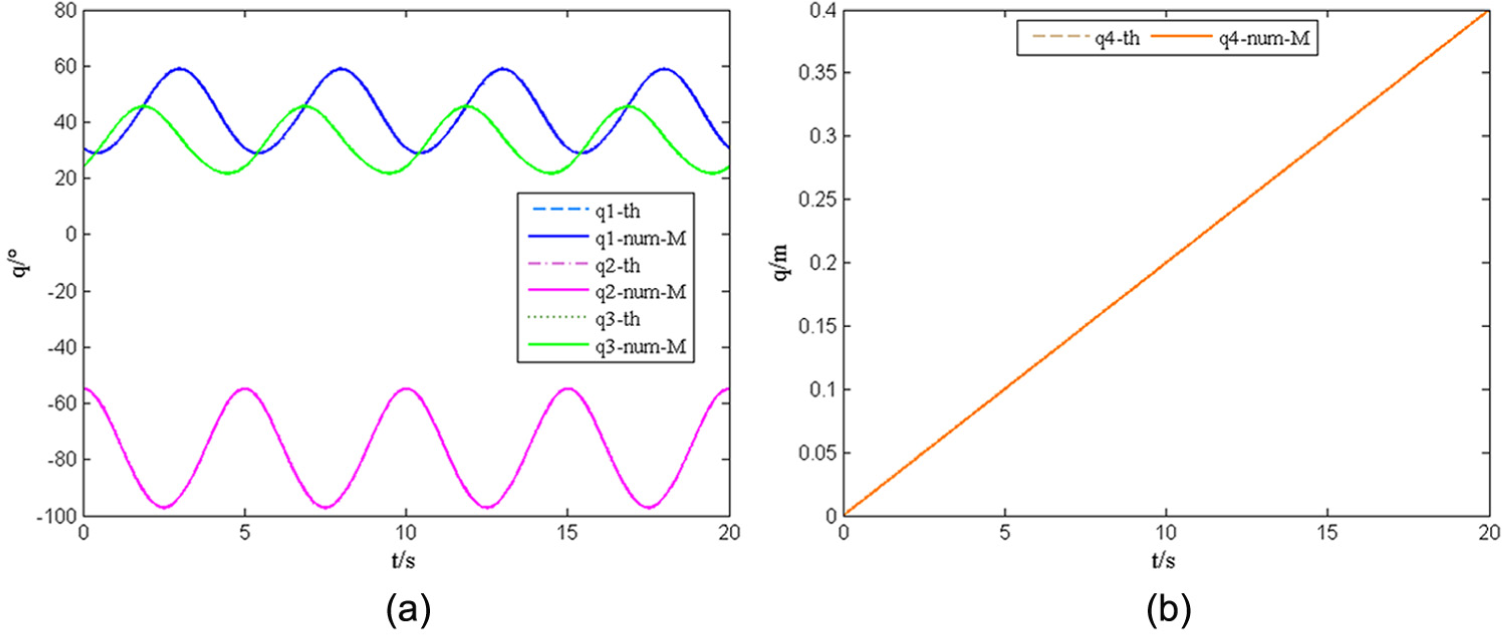
Comparisons of dynamic responses between numerical value and theoretical value: (a) q₁, q₂, q₃ and (b) q₄.

Figure 3.

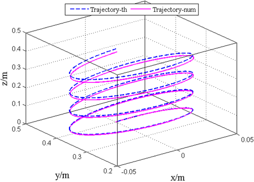
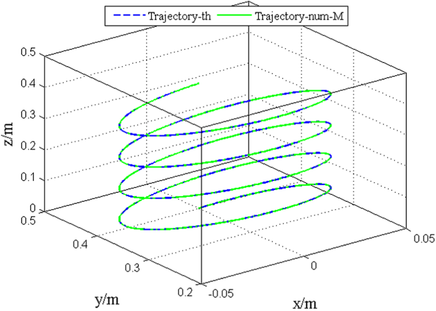
Comparison of the trajectories between numerical value and theoretical value.

Figure 4.

Sketch map of joint errors between numerical value and theoretical value: (a) $q_{1}$ -error, $q_{2}$ -error, $q_{3}$ -error and (b) $q_{4}$ -error.

Figure 5.

Displacement errors between numerical value and theoretical value: (a) x-error, (b) y-error, and (c) z-error.

Figure 2 represents the dynamic responses at each joint of the SCARA robot subjected to the space trajectory constraints, in which the solid curves and the dash curves represent the numerical value and the theoretical value, respectively. The numerical trajectories is slightly off the theoretical trajectory with time, as illustrated in Figure 3, in which the solid curve and the dash curve represent the numerical trajectory and the theoretical trajectory, respectively. However, the joint errors and displacement errors in the satisfaction of the constraints tend to increase in time and spoil reliability of the simulation results, as shown in Figures 4 and 5, respectively. The largest displacement errors correspond to about 8 × 10⁻⁴ m in x-axis, 7 × 10⁻³ m in y-axis, and 0.01 m in z-axis, which should not be neglected. Therefore, it is necessary to consider the numerical method for reducing the errors.

Error reducing

Constraint violation arises when the initial conditions are incompatible with the constraint equations. This makes the simulation results seriously different from real situations. Accordingly, it is necessary for the use of Baumgarte stabilization method to suppress constraint violation. In the standard formulation of the method, the (open-loop) second-order differential constraints, $\overset{\cdot\cdot}{Φ} = 0$ , are replaced with its stabilized (closed-loop) form²³

\overset{\cdot\cdot}{Φ} + α \overset{\cdot}{Φ} + β Φ = 0

(52)

in which $α = diag {α_{1}, α_{2}, \dots, α_{p}}$ and $β = diag {β_{1}, β_{2}, \dots, β_{p}}$ .

If $α_{i}, β_{i} > 0$ , $Φ$ approaches to zero asymptotically. Thus, from equation (52), a more general constraint equation is obtained, which nonetheless retains the form of equation (49).²² Thus, utilizing the Baumgarte stabilization method, the equations of motion for a system subjected to constraints are stated in the form

[\begin{matrix} M & - A^{T} \\ A & 0 \end{matrix}] [\begin{matrix} \overset{\cdot\cdot}{q} \\ λ \end{matrix}] = [\begin{matrix} Q \\ b - α \overset{\cdot}{Φ} - β Φ \end{matrix}]

(53)

Then, equation (52) yields the following constraint equation

\begin{matrix} [\begin{matrix} - l_{1} c_{1} - l_{2} c_{12} & - l_{2} c_{12} & 0 & 0 \\ - l_{1} s_{1} - l_{2} s_{12} & - l_{2} s_{12} & 0 & 0 \\ 1 & 1 & 1 & 0 \\ 0 & 0 & 0 & 1 \end{matrix}] [\begin{matrix} {\overset{\cdot\cdot}{q}}_{1} \\ {\overset{\cdot\cdot}{q}}_{2} \\ {\overset{\cdot\cdot}{q}}_{3} \\ {\overset{\cdot\cdot}{q}}_{4} \end{matrix}] = \\ [\begin{matrix} \begin{matrix} - {\overset{\cdot}{q}}_{1}^{2} l_{1} s_{1} - {({\overset{\cdot}{q}}_{1} + {\overset{\cdot}{q}}_{2})}^{2} l_{2} s_{12} - 0.05 \times (0.4 π)^{2} \sin (0.4 π t) \\ - α_{1} (- {\overset{\cdot}{q}}_{1} l_{1} c_{1} - ({\overset{\cdot}{q}}_{1} + {\overset{\cdot}{q}}_{2}) l_{2} c_{12} - 0.05 \times (0.4 π) \cos (0.4 π t)) \\ - β_{1} (- l_{1} s_{1} - l_{2} s_{12} - 0.05 \sin (0.4 π t)) \end{matrix} \\ \begin{matrix} {\overset{\cdot}{q}}_{1}^{2} l_{1} c_{1} + {({\overset{\cdot}{q}}_{1} + {\overset{\cdot}{q}}_{2})}^{2} l_{2} c_{12} - 0.05 \times (0.4 π)^{2} \cos (0.4 π t) \\ - α_{2} (- {\overset{\cdot}{q}}_{1} l_{1} s_{1} - ({\overset{\cdot}{q}}_{1} + {\overset{\cdot}{q}}_{2}) l_{2} s_{12} + 0.05 \times (0.4 π) \sin (0.4 π t)) \\ - β_{2} (l_{1} c_{1} + l_{2} c_{12} - 0.35 - 0.05 \cos (0.4 π t)) \end{matrix} \\ - α_{3} ({\overset{\cdot}{q}}_{1} + {\overset{\cdot}{q}}_{2} + {\overset{\cdot}{q}}_{3}) - β_{3} (q_{1} + q_{2} + q_{3}) \\ - α_{4} ({\overset{\cdot}{q}}_{4} - 0.02) - β_{4} (q_{4} + l_{0} - 0.02 t) \end{matrix}] \end{matrix}

(54)

Note that an improper choice of $α$ and $β$ can lead to unacceptable results in the dynamic analysis of the multibody systems.²⁴ Baumgarte¹⁹ highlighted that the suitable choice of $α$ and $β$ is performed by numerical experiments. For simplicity, we choose $α_{1} = α_{2} = α_{3} = α_{4} = 0.5$ and $β_{1} = β_{2} = β_{3} = β_{4} = 200$ . The simulation results are presented in Figures 6 –10.

Figure 6 represents the dynamic response curves as a function of time t between modified numerical value and theoretical value, in which the solid curves and the dash curves represent the modified numerical value and the theoretical value, respectively.

The trajectories are almost coincident by comparing between modified numerical value and theoretical value, as illustrated in Figure 7, in which the solid curves and the dash curves represent the modified numerical value and the theoretical value, respectively. The overall effect of constraint trajectory obtained by modified numerical integration gets clear improvement.

Comparing with the qi-error between numerical value and theoretical value, the amplitude of qi-error between modified numerical value and theoretical value is substantially lowered, as illustrated in Figure 8. Obviously, the errors are within an acceptable range that the constraint relations in x-, y-, and z-axis are being maintained well as desired, as depicted in Figure 9.

Figure 10 represents the constraint torques to make the SCARA robot follow the space trajectory for precise application.

Figure 6.

Comparisons of dynamic responses between modified numerical value and theoretical value: (a) q₁, q₂, q₃ and (b) q₄.

Figure 7.

Comparison of the trajectories between modified numerical value and theoretical value.

Figure 8.

Comparisons of joint errors for-and-aft modification: (a) $q_{1}$ -error, (b) $q_{2}$ -error, (c) $q_{3}$ -error, and (d) $q_{4}$ -error.

Figure 9.

Comparison of displacement errors between for-and-aft modification: (a) x-error, (b) y-error, and (c) z-error.

Figure 10.

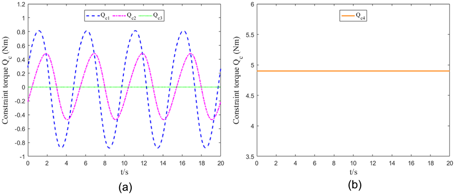
Constraint torques: (a) Qc1, Qc2, Qc3, and (b) Qc4.

Conclusion

Aiming at dynamic modeling of the SCARA robot subjected to constraint, this article establishes the dynamic equation based on the Udwadia–Kalaba theory and reduces the errors using Baumgarte stabilization method. The comparison of numerical simulations confirms the ease of implementation and the high numerical accuracy of this methodology. The research process reveals some conclusions as follows:

The desired space trajectory, which is regarded as constraints imposed on the system, is integrated into the dynamic modeling of the system dexterously.

The explicit, closed-form expression for the constraint torques required to guarantee the end-effector of the SCARA robot to move along the desired space trajectory and the explicit dynamic equation of the system without Lagrange multiplier are obtained.

Baumgarte stabilization method is used for constraint violation suppression to realize trajectory motion with high accuracy.

Footnotes

Academic Editor: Kai Bao

Declaration of conflicting interests

The author(s) declared no potential conflicts of interest with respect to the research, authorship, and/or publication of this article.

Funding

The author(s) received no financial support for the research, authorship, and/or publication of this article.

References

Zhao

Zhen

Chen

. Dynamic modeling and simulation of multi-body systems using the Udwadia-Kalaba theory. Chin J Mech Eng 2013; 26: 839–850.

Braun

Goldfarb

. Eliminating constraint drift in the numerical simulation of constrained dynamical systems. Comput Method Appl M 2009; 198: 3151–3160.

Kane

. Dynamics of nonholonomic systems. J Appl Mech 1961; 28: 574–578.

Korayem

Shafei

. A new approach for dynamic modeling of n-viscoelastic-link robotic manipulators mounted on a mobile base. Nonlinear Dynam 2015; 79: 2767–2786.

Udwadia

Kalaba

. A new perspective on constrained motion. Proc R Soc Lond A Math Phys Sci 1992; 433: 407–410.

Udwadia

Kalaba

. On the foundations of analytical dynamics. Int J Non Linear Mech 2002; 37: 1079–1090.

Udwadia

Kalaba

. What is the general form of the explicit equations of motion for constrained mechanical systems?J Appl Mech 2002; 69: 335–339.

Udwadia

Koganti

. Dynamics and control of a multi-body planar pendulum. Nonlinear Dynam 2015; 81: 845–866.

Udwadia

Wanichanon

. Control of uncertain nonlinear multibody mechanical systems. J Appl Mech 2014; 81: 041020.

10.

Udwadia

Wanichanon

. A closed-form approach to tracking control of nonlinear uncertain systems using the fundamental equation. Earth Space 2012; 10: 1339–1348.

11.

Udwadia

Wanichanon

Cho

. Methodology for satellite formation-keeping in the presence of system uncertainties. J Guid Control Dynam 2014; 37: 1611–1624.

12.

Liu

. Simple method to the dynamic modeling of industrial robot subject to constraint. Adv Mech Eng 2016; 8: 1–9.

13.

Huang

Chen

Zhong

. Udwadia-Kalaba approach for parallel manipulator dynamics. J Dyn Syst Meas Contr 2013; 135: 061003.

14.

Pennestrì

Valentini

de Falco

. An application of the Udwadia–Kalaba dynamic formulation to flexible multibody systems. J Franklin Inst 2010; 347: 173–194.

15.

Oprea

. A constrained motion perspective of railway vehicles collision. Multibody Syst Dyn 2013; 30: 101–116.

16.

Schutte

Dooley

. Constrained motion of tethered satellites. J Aerospace Eng 2005; 18: 242–250.

17.

Pappalardo

. A natural absolute coordinate formulation for the kinematic and dynamic analysis of rigid multibody systems. Nonlinear Dynam 2015; 81: 1841–1869.

18.

Sun

Zhao

Zhen

et al . Application of the Udwadia–Kalaba approach to tracking control of mobile robots. Nonlinear Dynam 2016; 83: 389–400.

19.

Baumgarte

. Stabilization of constraints and integrals of motion in dynamical systems. Comput Method Appl M 1972; 1: 1–16.

20.

Blajer

. Methods for constraint violation suppression in the numerical simulation of constrained multibody systems—a comparative study. Comput Method Appl M 2011; 200: 1568–1576.

21.

Murray

Sastry

et al . A mathematical introduction to robotic manipulation. Boca Raton, FL: CRC Press, 1994.

22.

Cho

Udwadia

. Explicit solution to the full nonlinear problem for satellite formation-keeping. Acta Astronautica 2010; 67: 369–387.

23.

Lin

Chen

. A PID type constraint stabilization method for numerical integration of multibody systems. J Comput Nonlin Dyn 2011; 6: 044501.

24.

Nikravesh

. Some methods for dynamic analysis of constrained mechanical systems: a survey. In: Haug

(ed.) Computer aided analysis and optimization of mechanical system dynamics. Berlin: Springer, 1984, pp.351–368.

Dynamic modeling of SCARA robot based on Udwadia–Kalaba theory

Abstract

Keywords

Introduction

Udwadia–Kalaba theory

Unconstrained multibody dynamics

Constraint description

Constrained multibody dynamics

Dynamic modeling of SCARA robot

Unconstrained dynamics

Result

Proof

Constraint description

Constraint torque description

Numerical simulations

Error reducing

Conclusion

Footnotes

Declaration of conflicting interests

Funding

References