
Abstract
A unit module of the mobile modular reconfigurable robot (M2rBot) with the 12 connection ways is first introduced. For expressing the spatial connection relations and the traversing paths of the M2rBot, a novel method of the automatic generation of the spatial connection matrix is presented based on our proposed double-module space pose transformation. The motion equations are also automatically generated to solve the reconstruction problems of mechanical configuration, kinematics, and dynamics. This method enables to analyze the kinematics and dynamics for both serial and multi-branch modular robots with different configurations. As for the control strategies, a fuzzy robust adaptive controller is also developed to adapt to the different configurations without adjusting any control parameters. The results show that the novel method is effective, and the proposed controller can satisfy tracking performances and quickly adapt to the change of the configurations, the frictions, and the external disturbances. The proposed method and controller are easy to extend to other modular robots.
Introduction
Modular reconfigurable robot (MRR), composed of multiple modular components, is a variable topology system that can manually rearrange the modules’ connectedness and form a large variety of robot configurations. Due to the versatility and the replace ability, the MRR would have a great potential application to meet varieties of task requirements in unstructured and dynamic environments.1–3 In a plain field, it can change its configuration into a loop to move fast. On the bumpy road, the robot can reconfigure itself into the four-leg or multi-leg shape to easily crawl over obstacles. The robot can also perform tasks that one single module or a fixed-structure robot cannot accomplish, and it can also append specialized units to the original configuration. The specialized units are grippers, welding guns, or sensor units such as cameras.
The MRR can be traced back to the CEBOT 4 introduced by Toshio Fukuda in the late 1980s and is divided into three categories: mobile architecture, lattice architecture, and chain architecture. 5 Utilizing the mobility, it can form the chain or the lattice architecture through the locking mechanism, and it can also implement more kinds of configurations. Several literatures of the mobile architecture were published, such as Trimobot, 6 UBot, 7 ModRED, 8 Scout robot, 9 AMOEBA, 10 Sambot, 11 360bot, 12 M2sbot, 13 and OMNIMO. 14 Previous researchers mainly focused on the structure design12–14 and the locomotion and control.6,7,9,15–17 However, the research of automatic generation of motion equations is not enough, and especially the configuration adaptive control is less.
The common kinematics methods are the Denavit–Hartenberg (D-H) method 18 and the product of exponential (POE) method. 19 Compared with the traditional D-H method, the POE method has more explicit geometric meaning and is more simple. Fei and Zhao 19 proposed the automatic generation of the forward kinematics for cuboid and cubic modules with POE and only analyzed the theoretical configuration of the reconfigurable mechanical system. Pan et al. 20 derived the forward kinematics of the multi-chain MRR with different joints, links, bases, and end effectors by the assembly incidence matrix (AIM) and the path matrix. The described methodologies in the above works, however, are useful only for the special configurations, and the assembly representation is also very complex. When the assembly sequences are changed, the automatic generation becomes difficult due to the large number of intermediate variables. Bi et al. 21 applied the specific finite element method (FEM) to the robotic configuration with serial, parallel, or hybrid structures. Each module was regarded as a conceptual element which could be predefined. The method simplified the number of variables, but the spatial expression was more complex than the above two.
For a fixed-configuration robot, the dynamics equations are generally derived by manual. However, it can be challenging and time-consuming to obtain the dynamics equation of each configuration on the MRR. It is impossible and impractical to derive and compute the dynamics equations of each configuration because the configuration cannot be known in advance. Yang 22 proposed one unified modeling method of the underwater self-reconfigurable robot based on graph theory and path matrix using Kane’s method. Djuric and ElMaraghy 23 provided any automatic generation of the dynamics equation matrices elements based on Newton–Euler method. The calculated parameters were all computed containing the joint position, velocity, acceleration, and input torque or forces. Fei et al. 24 presented a compensative and recursive method for generating the dynamics equations automatically. The dynamics parameters could not be accurately computed with the compensative method. The dynamics equations based on Newton–Euler method are simple, fast, and precise, but the forward and inverse recursive equations destroy the whole structure of the dynamics model, so it is difficult to design the compensation controller.
The generated dynamics model is a nonlinear model. There are different possibilities to deal with nonlinearity either using Jacobi linearization or compensating the nonlinear terms through feedback techniques. One of the most used methods is to linearize the model at a certain operation point by use of Jacobi method. In recent years, the compensatory control method has attracted lots of researches and probably becomes the first choice.25,26 Compared with the Jacobi method, the compensatory control method is to more precisely approximate the model uncertainty terms. For the MRR, the compensatory controller is designed not only for compensating uncertainties of one fixed-configuration model but also for adapting to the dynamics models with different configurations. The research on compensating uncertainties of different dynamics models using one single controller is a huge challenge, especially without adjusting any control parameters.
In this article, the main researches based on the above problems include the following. To solve the kinematics generation problem of multiple connection ways, a unique double-module space pose transformation (DMSPT) based on the screw form is first proposed. Second, inspired by the work from Chen and Yang, 27 the kinematic and dynamics equations for multiple branches are derived by the recursive method with a more simple expression of spatial connection relationships among the modules. In order to avoid destroying the whole structure of the dynamics models, the closed-form dynamics equations can be derived according to different configurations. And then, a fuzzy robust adaptive controller is presented, which contains a feedback plus a robust term for the model uncertainties, frictions, and external disturbances. Finally, the simulation results are implemented to verify the effectiveness of the proposed controller for the motion equations of different configurations without adjusting any control parameters and to compensate simultaneously the frictions and external disturbances of different configurations.
M2rbot unit module description
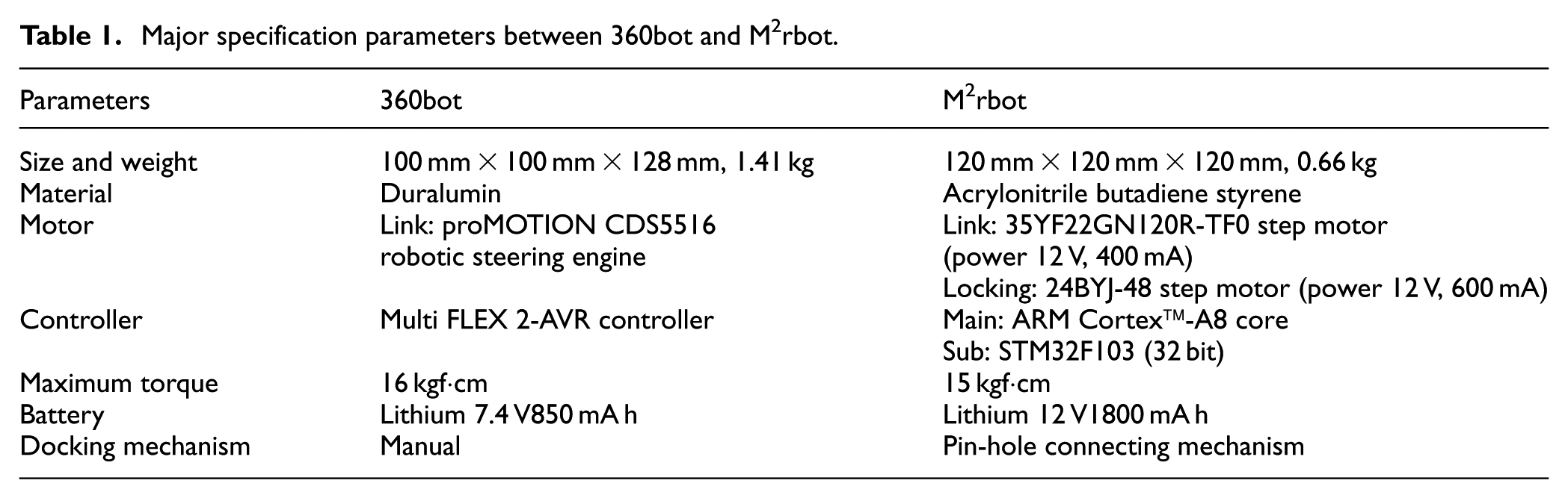
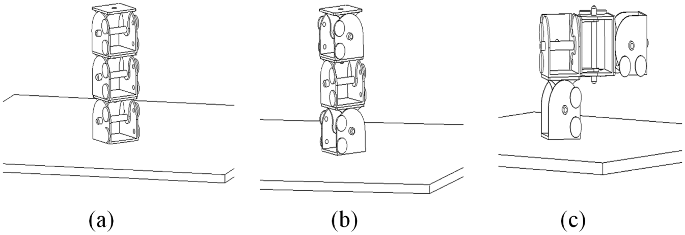
For the M2rbot, the following characteristics are considered: the simple module structure which can move independently, the rich connecting surfaces and connecting ports, and the reliable locking mechanism. The basic design of the M2rbot is identical to the former 360bot 12 and M2sbot 13 as shown in Figure 1. The M2rbot has similar sizes and similar physical properties to the 360bot and M2sbot, but it can be more firmly locked and be less weight. The robot has a slight mobile ability to adapt to the ground, and it can realize a reliable physical connection between modules. Table 1 summarizes the major specification parameters between the 360bot and the M2rbot.
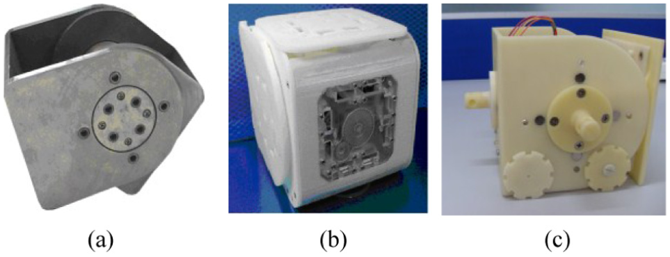
Developed modular robot: (a) 360bot, (b) M2sbot, and (c) M2rbot.
Major specification parameters between 360bot and M2rbot.
The M2rbot unit module is shown in Figure 2. It mainly comprises two U-type blocks and a rotating shaft. The inner Ub block can independently rotate around the shaft by ±90°. The Ub is used as the active connection surface (C1) to connect with the adjacent module. The outer Ua block has three passive connection surfaces (C2, C3, and C4) which to be connected with the other adjacent modules. Viewed from the top, the three passive surfaces are sequentially defined in a counter-clockwise direction. Although the three passive surfaces are not identical, they can be connected symmetrically in four possible connection ports and it can achieve more topological configurations. The typical topology configurations consisting of some modules are shown in Figure 3. With the increase in the modules, the number of configurations will increase exponentially.
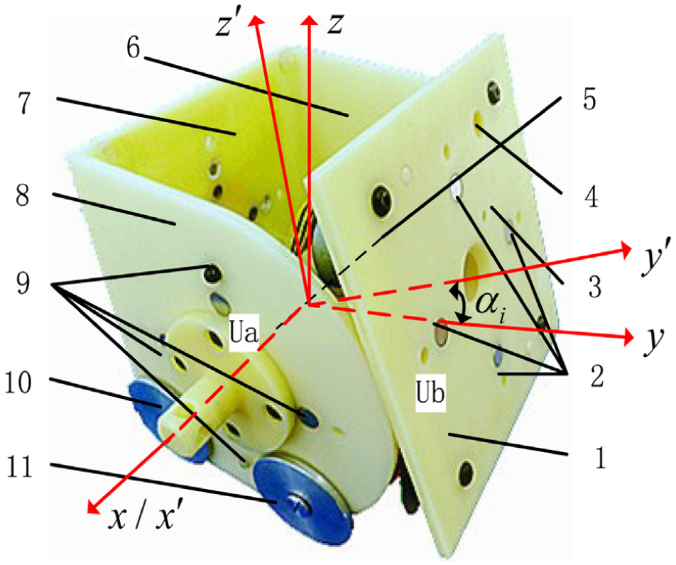
M2rbot unit module.
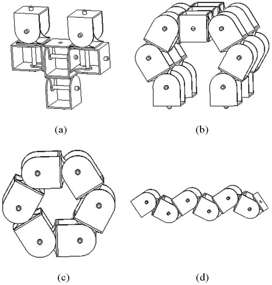
Different configurations of M2rbot: (a) double-branch configuration, (b) quadruped configuration, (c) ring configuration, and (d) snake configuration.
All blocks are connected by dyads (a dyad is defined as two adjacent modules connected through a passive block and an active one). The dyad structure of the M2rbot unit module has the following properties. (1) Each block is always a neighbor of opposite block as a dyad. (2) The dyad has four connection ports, which can provide more rich connection configurations.
Module assemblies and kinematic generation
The unit modular robots can bring some possible assembly sequences. The kinematics varies according to the different configurations and assembly sequences between the modules. For the M2rbot, the kinematics starts with a two-module assembly model and a spatial connection matrix (SCM) representation.
Two-module assembly model
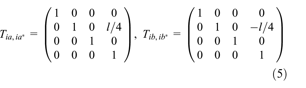
A unit module of the M2rbot can be simply abstracted as the model with two rigid bodies and a rotating shaft. The Ua of the ith module is noted as ia and the Ub as ib. As shown in Figure 2, the center point of the rotation shaft is the origin of the

where
There are 12 different connecting dyads for the DMSPT as listed in Table 2. The connected dyad between the connector

where k denotes the passive connector of module j,
Double-modules space pose transformation (DMSPT).
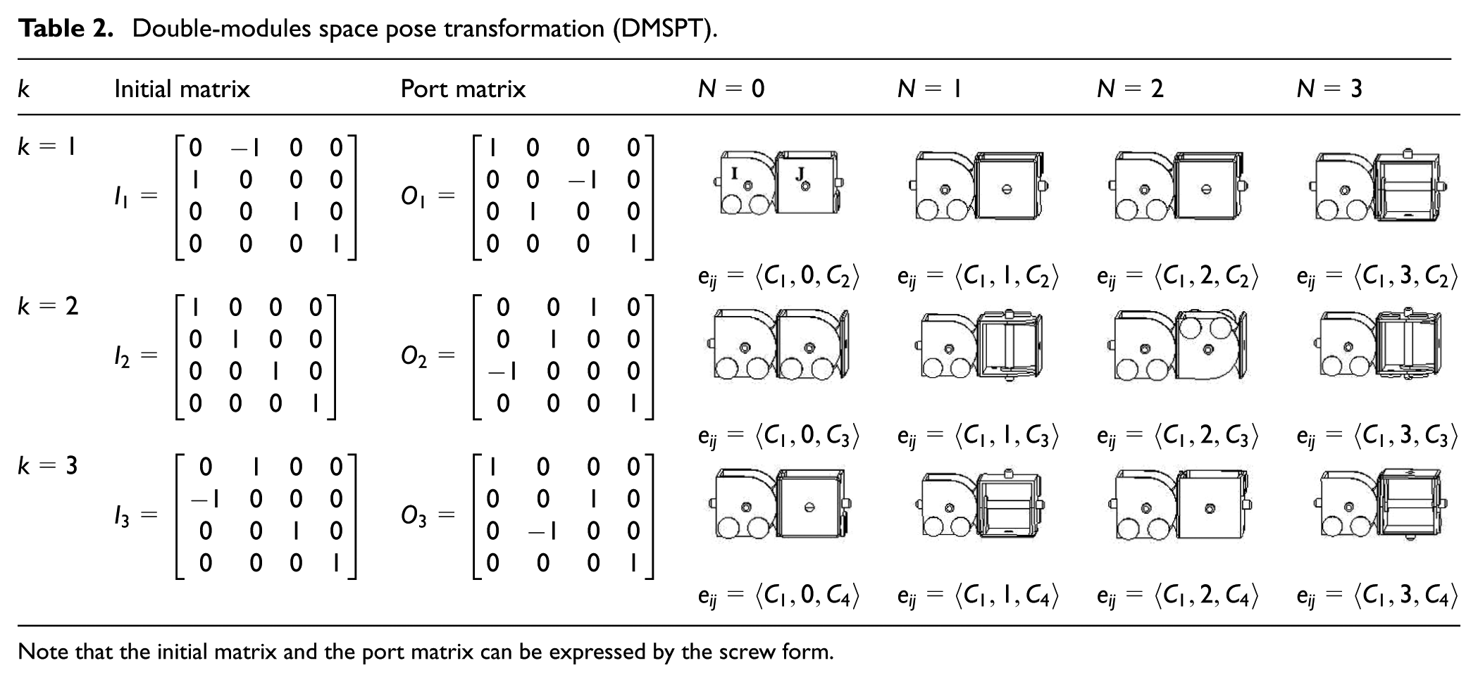
Note that the initial matrix and the port matrix can be expressed by the screw form.
SCM representation with a branching structure
The assembly of multiple modules can represent not only a simple chain structure but also a complicated branching structure. When a base module is determined at a chain structure, the transformation order of the module starts from the base module. For a branching one, the shortest traversing paths can be obtained using the breadth-first search (BFS) or the depth-first search (DFS) algorithms. Note that the kinematics of a closed-loop configuration requires additional constraints and is not considered here.
The SCM, similar to a kinematic graph as a kinematic chain, is proposed for representing the spatial assemblies between the modules and their neighbor modules. A huge advantage of the SCM representation method is that one smaller matrix is only needed to store the spatial assemblies, and there is a one-to-one relationship between the spatial assemblies and the SCM. Compared with the AIM, 27 the kinematics calculation can be done simultaneously for all branches by the SCM containing the traversing paths. The double-branch configuration in Figure 3(a) can be depicted as shown in Figure 4. The graph differs from an ordinary graph since it can express the connector directions. The directions can be expressed from the active connectors to the passive ones. The SCM can also be represented by a vertex-edge matrix. Furthermore, in order to adapt to the recursive kinematics, an additional row and additional column are inserted to the matrix for the joint angles and the connecting ports. The six-module configuration with two branches in Figure 4 can be obtained as follows.


Kinematic graph representation.
This SCM can provide a flexible way to calculate the sequences of all possible transformations along the traversing paths during run time. For a branching configuration, the forward kinematics can be obtained from a chosen base module to each end link in all branches. The forward kinematic transformations for the path k with m branches, based on the dyad kinematics, can be formulated as follows

where
Robot dynamics modeling
Dynamics for the links assembly
The rotation shaft of the unit module is considered as “joint.” The Ua locked with one Ub or more is considered as “links.” Let the links ia and ib be the two links connected by joint i. If the two or more adjacent modules are rigidly connected, we consider the connection of joint i and link i as the links assembly i. Taken the six-module robot configuration with two branches as an example, the link assembly of the robot is shown in Figure 5.

Link assembly of six-module configuration.
Suppose frame i is the body (or local) coordinate frame. The mass frame i* can be located on the mass center of the links assembly. In general, the two coordinate frames do not coincide with each other. The two frames belong to the same rigid link assembly, and then, for the ith unit module, we can get following
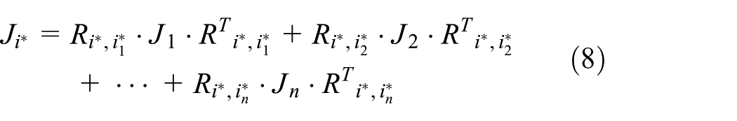
Suppose links assembly i is composed of one joint i and more links, for a branched structure,
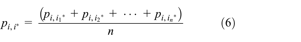
where n denotes the number of the links, and there are
where
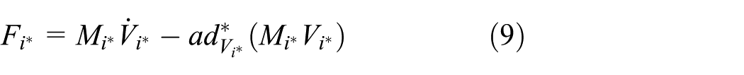
where

Equation (9) is not relative to the above kinematic equation of the body frame, so it must be transformed to the body frame i. So, we use the following identities
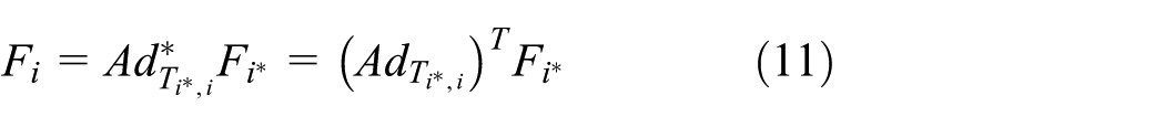


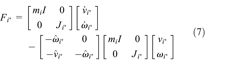
Substituting equations (11)–(13) into equation (9), and using equation (14), Newton–Euler equation of generalized link assembly i with respect to the body frame i can be rewritten as follows

where
Newton–Euler recursive equation
The first considering point of the MRR is that the dynamics model of the robot assembly cannot be known a priori. Therefore, the robot should be able to generate its own equations autonomously without human intervention. The original idea for recursive equations and its closed forms were introduced by Chen and Yang. 27 In this article, starting with the SCM that contains all the information how to be assembled, the equations of motion can be done by following steps. Starting from the base module to end actuators, the SCM is gradually filled based on path search algorithms such as BFS or DFS. After the SCM is built and all paths are determined, the recursive equations can be started to be calculated.
The forward recursive velocity and acceleration can be written as follows
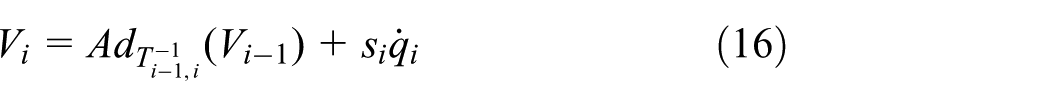

As for the backward iteration, equation (15) can be written in the following form
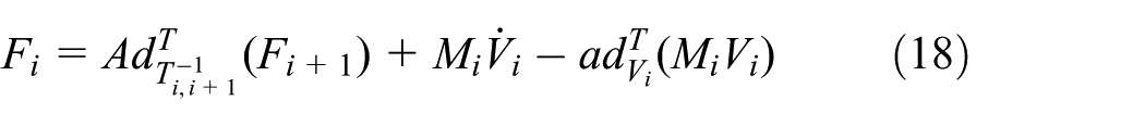

where
Closed-form equations of dynamics
By expanding Newton–Euler equations (16)–(19) in the body coordinates, the generalized velocity, generalized acceleration, and generalized force equations can be obtained from the following global matrix representations


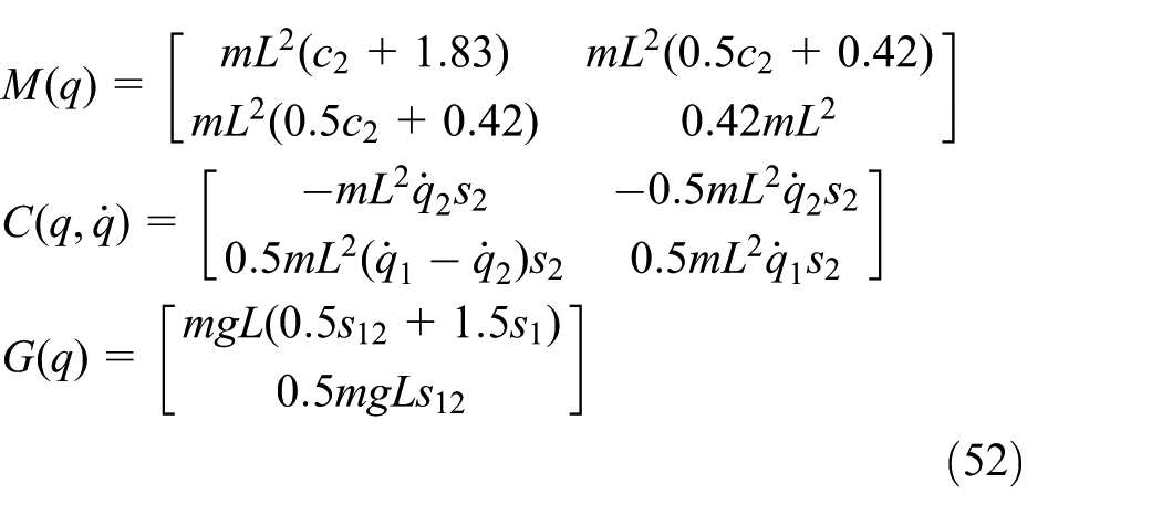
Substituting equations (20)–(22) into equation (23), we can obtain the closed-form equations of dynamics for a branching structure with (n + 1) modules

where


where
Configuration adaptive control
Previous researchers have focused on the dynamics modeling and the compensatory control method for a fixed configuration, and the researches of the configuration adaptive control for the MRR have been less in the past years. It is difficult to compensate the different model uncertainties without adjusting any control parameters. To deal with approximation errors, external disturbances, and frictions on different models, the adaptive fuzzy controller is appended by a robust compensator. For practical purposes, the controller may be applicable for the MRR due to dealing with the complex systems and implementing the controller without any precise knowledge of the exact dynamics model.
According to equation (24), the dynamics of the MRR incorporating the external disturbance and the friction can be represented by the following form

where
Rewriting equation (28), the equation can be shown as follows

Let us suppose

Substituting equation (30) into equation (29), we can get the following

Define

where
If the nonlinear function

where
Let us suppose

where


where

Up to now, even though the control law (34) is always well defined, it cannot guarantee the stability of the robot’s closed-loop system alone. The reason is partly due to the unavoidable unfixed errors of the unknown function


where

To meet the control objectives, the adaptive parameter


Substituting equations (39)–(43) into equation (32), we get the following

The following Lyapunov function can be defined by
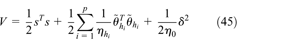
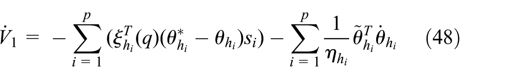
Differentiating equation (45), we can get the following

Substituting equation (44) into equation (46), the equation can be obtained as follows

where
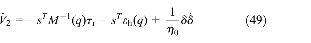
Substituting equation (42) into equation (48), we can obtain

It is clear that
By integrating equation (50) from

where
Using Barbalat’s Lemma,
28
we can have a conclusion that
Simulation results
To evaluate the automatic generation of motion equations, an example of the six-module configuration with two branches has been implemented.
29
Another example with one branch of the three different configurations can also be automatically generated. The proposed adaptive controller is applied to the second example as shown in Figure 6. The end module of the branch can be supposed as the terminal actuator without rotating. Therefore, the configurations (a) and (b) shown in Figure 6(a) and (b) have the same two degrees of freedom (DOFs), but its connection ports are different. The configuration (c) shown in Figure 6(c) has three DOFs. Once the SCMs and the parameters of the module (
Configuration (a)
Configuration (b)

Configuration (c)

where
Three different configurations with one branch: (a) 2 DOF configuration with the same connection way, (b) 2 DOF configuration with the different connection way, and (c) 3 DOF configuration with the different connection way.
The control objective is to force the joint outputs

The robot’s initial conditions are
The simulation results of configuration (a) without the friction and disturbance are shown in Figure 7, and those with the friction and disturbance are also shown in Figure 8. The results for configurations (b) and (c) with the same friction and disturbance are shown in Figures 9 and 10, respectively.
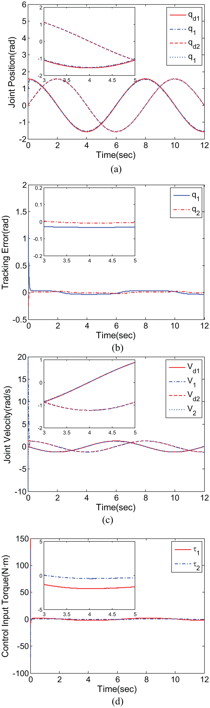
Configuration (a) without

Configuration (a) with

Configuration (b) with

Configuration (c) with
For configuration (a), we can see that the desired and actual trajectories shown in Figures 7 and 8 almost overlap with each other regardless of the frictions and disturbances. When the sudden friction and disturbance appears, the tracking trajectory has almost no change and the proposed control method can rapidly adapt to the sudden changes. But the tracking error, the joint velocity, and the input torque are affected by the sudden disturbance. When the sudden disturbance passed, the above results can quickly restore. Comparing Figure 7(b) with Figure 8(b), we can see that the tracking errors are quickly converging into a small limit area near zero.
From Figures 9 and 10, we can see that the actual outputs can similarly track the desired trajectories with two different configurations. Therefore, the control method can approximate the dynamics equations with the unknown terms. Because the tracking errors are quickly converging into a small limit area near zero, the algorithm can adapt to the different configurations. From Figures 8 to 10, the joint tracking errors, based on the periodic disturbances
From these local amplification diagrams, the response curves are clearer to be seen. It can be shown that the control method can effectively compensate the whole unknown terms. The tracking velocities will almost overlap the desired velocity except for the time area
In the actual experiment, more mechanistic interferences are needed to be considered such as the increment in the torque caused by the friction, the mechanical and communicational delay, the vibration caused by the two adjacent modules to be unstably locked and the decrease in the control performance caused by the system modeling errors.
Conclusion
In this article, a novel method for automatic generation of motion equations is proposed for the multi-branch MRR, and the fuzzy adaptive robust controller with adapting the different configurations is also presented. The method enables to analyze the kinematics and dynamics of modular robots, and the adaptive controllers are also implemented for both the serial and the multi-branch configuration with different connectors and different connecting ports by the DMSPT. The dynamics equations of both the serial and the multi-branch configuration are derived by the Newton–Euler recursive method. Therefore, when the SCM is input, the dynamics equations can be automatically generated. Different examples are used to evaluate the serial and the multi-branch configurations. The proposed fuzzy adaptive robust controller can compensate the dynamics model uncertainties of different configurations. The simulation results can not only illustrate the effectiveness on tracking performance, but also it quickly adapt to the change in the configurations, the frictions, and the external disturbances. The method will be used to the reconfigurable fixture system in the sheet metal assembly line for the automotive industry, which can satisfy the ever-increasing demand for automotive product variety as well as shortens the product changeover time. We will also replace the end effectors of the robot for adapting the different tasks, that is, wielding or grinding.
Footnotes
Academic Editor: Seiichiro Katsura
Declaration of conflicting interests
The author(s) declared no potential conflicts of interest with respect to the research, authorship, and/or publication of this article.
Funding
The author(s) disclosed receipt of the following financial support for the research, authorship, and/or publication of this article: This work was supported by National Natural Science Foundation of China (61503119 and 61473113) and by Tianjin Natural Science Foundation of China (15JCY BJC19800, 15ZXZNGX00090, and 16JCZDJC 30400).