Sage Journals: Discover world-class research

Abstract

Indoor testing should reproduce the real-world environment in order to be effective. In this article, an efficient methodology to reproduce road profiles on a four-poster rig is presented: such a method includes a complex rig control strategy based on an iterative process. Road profiles come from a purposely designed set of sensors fitted on the car which remains the same regardless of the vehicle or surface type. Particular stresses such as speed humps, potholes and manholes can be reproduced as well. Since there are no previous similar studies, a validation is provided by comparing road and rig data streams and using the maximum absolute error and root mean square error as performance indexes. Results show that the rig is able to reproduce road profiles and the related inputs to the vehicle successfully; hence, the method is reliable and effective.

Keywords

Road reproduction indoor testing durability tests four-poster test rig chassis and suspensions testing vehicle ride testing

Introduction

Outdoor testing is the best way to prove the reliability of a vehicle in terms of chassis and suspension durability. However, long-term road tests are time-consuming and expensive. As a matter of fact, current vehicles show a very low failure probability, for example, 3.53 × 10e−5 at 30 × 10e+4 km.¹

Indoor testing is now a consolidated activity, considered complementary to traditional road testing. Usually, indoor chassis/suspension tests are performed in dedicated laboratories by means of very sophisticated rigs and equivalent or accelerated excitations. According to Shafiullah and Wu,² a 95% accuracy can be achieved this way with regard to fatigue and durability tests.

However, sometimes even more accurate tests are required in order to achieve fully reliable results. In particular, special applications such as motorsport and military vehicles require a very precise prediction of their life expectancy, either on the full vehicle or on systems and components. Accurately reproducing the road input time history on an indoor test rig is considered a good strategy to get a reliable fatigue characterization while saving time and money, as reported in Uberti et al.³ Repeatability is also a significant advantage with lab testing.

Road profile reproduction on the four poster can be used for other purposes as well; the literature shows that it is a key device to evaluate the friction performance of a suspension system⁴ and its behaviour as far as kinematics and compliance are concerned.⁵ Comfort evaluations can also be performed allowing physicians and engineers to better understand musculoskeletal and/or physiological issues occurring on people driving commercial vehicles, trucks and agricultural vehicles,^3,6–8 while some studies^9–11 show that a four poster can perform the same evaluations on motorcycles by means of a purposely designed fixture. Studies^9,12,13 also state that the four-poster rig has become a reference in the field of motorcycle testing.

Apart from durability, the four poster is also used for many other types of testing such as noise vibration and harshness (NVH),¹⁴ ride comfort,^15,16 investigation of frequency response and vibration modes with resonance tracking^17,18 on full vehicles, systems and single components. It has also been used for the optimization of vertical dynamics (e.g. for damping fine tuning) and for active and semi-active suspension testing.¹⁹ This sort of testing is particularly suitable for the validation of simulation models. In the motorsport area, a so-called seven-poster rig (i.e. a four poster with additional actuators for aerodynamic downforce and lateral load transfer) is often employed for setup optimization, typically to achieve a stable aerodynamic platform and/or minimize tyre contact patch load variations, or even just to measure real-world suspension stiffness, damping and friction as well as structural stiffness properties. Inputs like a displacement sine sweep, a ramp or step can be used as well as full circuit lap time histories.^4,13

This article presents a methodology to record and accurately reproduce real-world road surface profiles, which are needed as inputs for indoor testing especially when particular care about accuracy in reflecting real-world conditions is required. First, the road surface profile to be reproduced should be recorded using the same vehicle to be tested. A set of sensors composed of accelerometers and linear displacement transducers is required in order to describe road inputs. One accelerometer is fitted on each wheel upright and a linear displacement transducer is fitted on each corner to measure suspension travel. The installation of such a set of sensors is meant to be simple and straightforward. Data are logged by means of a professional portable acquisition system and the sensor set remains the same no matter which is the car or the test surface. Acceleration and displacement data obtained are used as a reference for the test rig closed-loop control system, where vehicle-mounted sensors are part of the feedback line as described in section ‘Software configuration’.

The test bench itself is a servo-hydraulic four-poster rig, composed of four actuators which are closed-loop controlled as well, where the controlled variable is the piston shaft displacement along the vertical axis for each vehicle corner. This control loop is part of a complex iterative control system together with a system identification strategy and the servo-hydraulic actuators controls.

From 1976 onward, when Cryer et al.²⁰ first published their strategy for controlling a four poster for vehicle testing, iterative control applied on automotive test rigs is well known in the literature.^21–23 This kind of control has been chosen among others^24–26 because it features important advantages. For example, each cycle starts and ends in a steady-state condition and the target signals do not have to be targets for the closed-loop controller variables as reported in Plummer.²²

A validation is hence reported in the results section by comparing ‘real-world’ data from road acquisitions with ‘reproduced’ data from the test rig. Results show a very low root mean square (RMS) error between the two data streams. The difference between actual and reproduced values is always well under 1%, hence confirming effectiveness, accuracy and reliability of the proposed method. This ability to reproduce the road environment accurately on a laboratory test rig gives the development engineer a powerful tool to reduce the time to market.

This article is organized as follows. The test rig is briefly presented in section ‘The test rig’. Section ‘Materials and method’ aims at clarifying the rig control strategy and methods, including the procedure to obtain road profiles with a simple set of sensors, while a comparison between road data and reproduced data is shown in section ‘Results and discussion’. Conclusion remarks are finally given in section ‘Conclusion’.

The test rig

The so-called four-poster rig is generally used to excite an unrestrained road vehicle through the tyres in order to determine some of the dynamic characteristics of the vehicle, with particular regard to the suspension system. The excitation can be:

fed in terms of heave, roll and pitch,

aimed at resonance frequency tracking,

aimed at reproducing an acceleration/load history versus time as recorded in road testing.

It is composed of four pedestals based, servo-hydraulic linear actuators running on low-friction, hydrostatic bearings. Each vehicle tyre contact patch rests on a platform bolted to the actuator shaft. The actuators are bolted on a seismic base and adjustable in both the longitudinal and lateral directions to accommodate as many different vehicles as possible within a certain wheelbase and wheel track range. Each actuator is driven by three servo-valves and equipped with a membrane-type accumulator to deal with pressure spikes.

The whole system is fed by its own hydraulic control unit while the main power unit is equipped with a 150 kW electric motor and operates at 210 bar continuously and up to 400 bar for a limited amount of time. A feedback signal is provided by a high-precision position sensor (linear variable differential transformer (LVDT) type) fitted in an oil-tight compartment inside each actuator shaft. Table 1 reports the actuators main specifications, while Figure 1 shows the test rig layout and its main components.

Table 1.

Test rig specifications.

	Specification
Piston rod diameter	80 mm
Stroke	150 mm
Rated force capacity	40 kN
Operating pressure	210 bar
Transducer	LVDT
Accumulators	Pressure: 1 L, Return: 0.5 L

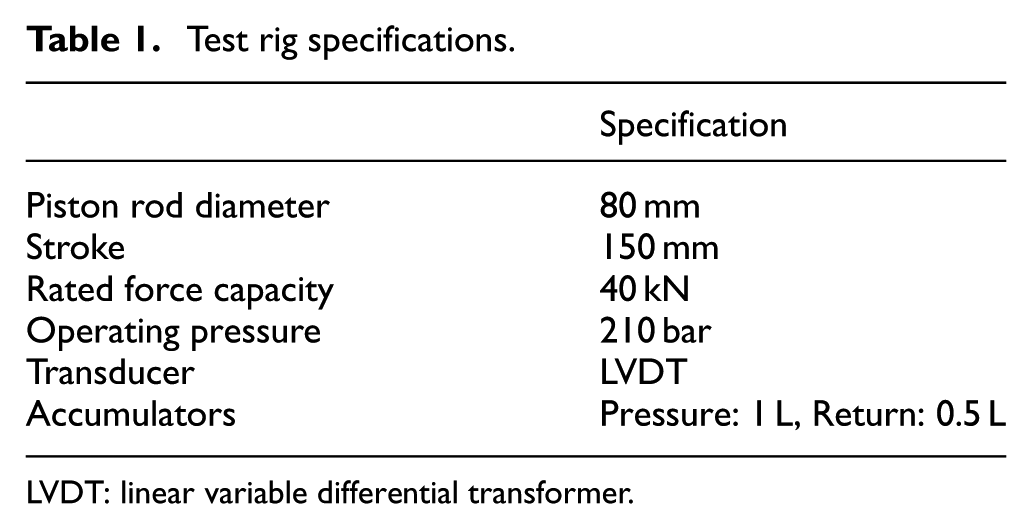
LVDT: linear variable differential transformer.

Figure 1.

Four-poster rig.

Materials and method

Control system hardware setup

Excluding the actuators themselves there are three key elements to the controller hardware layout. The first is the computer; this provides the main interface software, running under Windows^® operative system.

Inside the computer, there is a digital signal processing (DSP) card which provides real-time data acquisition and control for the system. This is linked via a ribbon cable to the controller chassis, which contains 16 digital I/O cards and 16 analogue I/O cards. The controller is then linked to the actuators themselves and any transducers on the rig, including those mounted on the test vehicle (see Figure 2 for the control hardware high-level schematics).

Figure 2.

Control system high-level schematics.

Software configuration

Road reproduction is the process where real-world road profile data are duplicated on the test rig. The proprietary control system is designed to give the operator access to power unit control, programming, system control and data processing in an integrated software front-end.

Figure 3 shows the key elements in the simulation process and how the controller guides the system through a drive file. Normally, the actuator control variable is the displacement. Four proportional–integral–derivative (PID) controllers acting in closed-loop and using the built-in LVDT transducer (see Table 1 and Figure 1) as a feedback line drive the position of each actuator.

Figure 3.

Simulation process layout.

Synchronized data acquisition and control signal generation capabilities enable an advanced form of de-convolution process (see equations (7) and (8)) to identify the system and then produce test rig controller drive files, as explained in Figure 4. The key elements of this process are the expected response, the actual system response measured through the above mentioned suspension motion transducers and the inverse system model.

Figure 4.

Iteration loop scheme.

Theoretically, if a test system is perfectly linear, the test rig drive file could be generated in just a single pass through the loop shown in Figure 4. However, real-world, non-linear systems and inevitably noise require the test rig drive signal to be generated with more than one pass through the control loop. The number of iterations required to generate the desired output depends on the ‘gain’ settings of the control loop and on the accuracy of the system model. Such a gain is a control parameter acting only on the road reproduction strategy without affecting the actuator control strategy (PID).

Table 2 reports the PID tuning parameters used to vibrate a front-engined car (see section ‘Road profiles and test vehicle’). The difference between the front and rear axle actuator pairs in terms of PID parameters is due to the front-biased weight distribution of the car.

Table 2.

PID’s tuning parameters.

Parameter	Symbol	Gain values
Parameter	Symbol	Front	Rear
Proportional	Kp	715	655
Integral	Ki	397	342
Derivative	Kd	188	160

System model

The first step in the iterative road reproduction process – reported in Figure 4– is to create a mathematical model of the system and the system matrix. The model includes the test rig, test vehicle and all the control hardware and response transducers. In order to create the model, a white noise signal is used to excite the test rig and the resulting test response is collected. The white noise drive file and the test system response file are then used to create a general system model, or matrix. Finally, an inverse form of the model, called the inverse system matrix, is calculated; this is then used to generate a trial test rig drive file required to achieve the expected response. Referring to Figure 5, the complete system mathematical model involved in the process is presented in the following equations:

Pitch movement of sprung mass

\begin{matrix} I_{yy} \cdot \overset{\cdot\cdot}{φ} - a \cdot c_{1} \cdot (x {\overset{\cdot}{m}}_{1} - {\overset{\cdot}{x}}_{1}) - a \cdot c_{2} \cdot (x {\overset{\cdot}{m}}_{2} - {\overset{\cdot}{x}}_{2}) \\ + b \cdot c_{3} \cdot (x {\overset{\cdot}{m}}_{3} - {\overset{\cdot}{x}}_{3}) + b \cdot c_{4} \cdot (x {\overset{\cdot}{m}}_{4} - {\overset{\cdot}{x}}_{4}) \\ - a \cdot k_{1} \cdot (x m_{1} - x_{1}) - a \cdot k_{2} \cdot (x m_{2} - x_{2}) \\ + b \cdot k_{3} \cdot (x m_{3} - x_{3}) + b \cdot k_{4} \cdot (x m_{4} - x_{4}) = 0 \end{matrix}

(1)

Roll movement of sprung mass

\begin{array}{l} I_{x x} \cdot \overset{\cdot\cdot}{θ} + \frac{t}{2} \cdot \\ [c_{1} \cdot (x {\dot{m}}_{1} - {\dot{x}}_{1}) + c_{3} \cdot (x {\dot{m}}_{3} - {\dot{x}}_{3}) - c_{2} \cdot (x {\dot{m}}_{2} - {\dot{x}}_{2}) \\ - c_{4} \cdot (x {\dot{m}}_{4} - {\dot{x}}_{4}) + k_{1} \cdot (x m_{1} - x_{1}) + k_{3} \cdot (x m_{3} - x_{3}) \\ - k_{2} \cdot (x m_{2} - x_{2}) - k_{4} \cdot (x m_{4} - x_{4})] = 0 \end{array}

(2)

Vertical movement of sprung mass (heave)

\begin{matrix} m \cdot x \overset{\cdot\cdot}{m} + c_{1} \cdot (x {\overset{\cdot}{m}}_{1} - {\overset{\cdot}{x}}_{1}) + c_{2} \cdot (x {\overset{\cdot}{m}}_{2} - {\overset{\cdot}{x}}_{2}) \\ + c_{3} \cdot (x {\overset{\cdot}{m}}_{3} - {\overset{\cdot}{x}}_{3}) + c_{4} \cdot (x {\overset{\cdot}{m}}_{4} - {\overset{\cdot}{x}}_{4}) + k_{1} \cdot (x m_{1} - x_{1}) \\ + k_{2} \cdot (x m_{2} - x_{2}) + k_{3} \cdot (x m_{3} - x_{3}) \\ + k_{4} \cdot (x m_{4} - x_{4}) = 0 \end{matrix}

(3)

Vertical movement of each corner (unsprung mass)

\begin{array}{l} m_{i} \cdot {\overset{\cdot\cdot}{x}}_{i} - c_{i} \cdot (x {\dot{m}}_{i} - {\dot{x}}_{i}) - k_{i} \cdot (x m_{i} - x_{i}) \\ + k t_{i} \cdot (x_{i} - u_{1}) = 0, i = 1, 2, 3, 4 \end{array}

(4)

Figure 5.

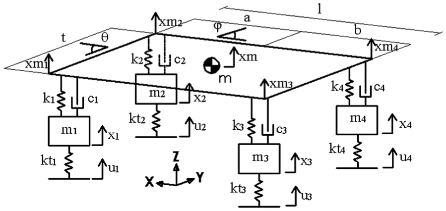
Complete system model scheme.

Please note that m is the sprung mass of the vehicle while $m_{i}$ are the four unsprung masses. $c_{i}$ are the dampers friction coefficient, $k_{i}$ are the suspension stiffness values while $k t_{i}$ represents the tyre vertical stiffness. Finally, $I_{xx}$ and $I_{yy}$ are respectively the sprung mass roll inertia and pitch inertia.

Considering now the general form of a state-space model, equations from equations (1) to (4) can be expressed in the space-state form as follows

\overset{\cdot}{x} (t) = A \cdot x (t) + B \cdot u (t)

(5)

The state vector is therefore

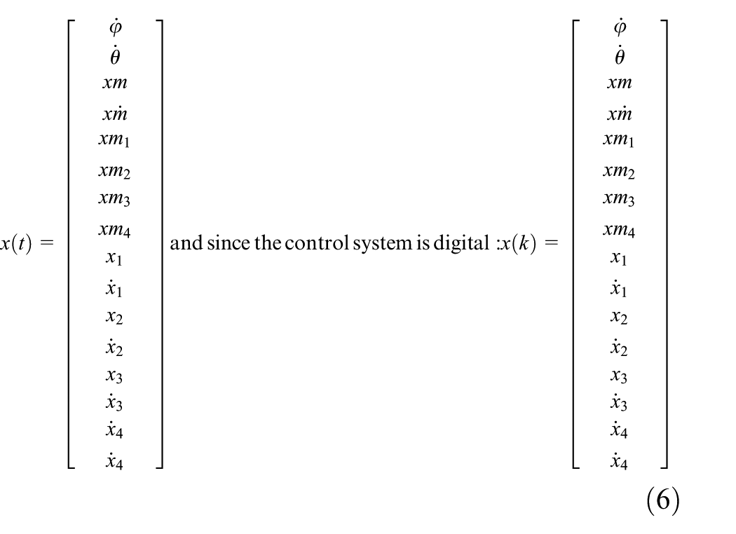
x (t) = [\begin{matrix} \dot{φ} \\ \dot{θ} \\ \begin{matrix} x m \\ \dot{x m} \\ \begin{matrix} x m_{1} \\ x m_{2} \\ \begin{matrix} x m_{3} \\ x m_{4} \\ \begin{matrix} x_{1} \\ {\dot{x}}_{1} \\ \begin{matrix} x_{2} \\ {\dot{x}}_{2} \\ \begin{matrix} x_{3} \\ \begin{matrix} {\dot{x}}_{3} \\ \begin{matrix} {\dot{x}}_{4} \\ {\dot{x}}_{4} \end{matrix} \end{matrix} \end{matrix} \end{matrix} \end{matrix} \end{matrix} \end{matrix} \end{matrix} \end{matrix}] and since the control system is digital : x (k) = [\begin{matrix} \dot{φ} \\ \dot{θ} \\ \begin{matrix} x m \\ \dot{x m} \\ \begin{matrix} x m_{1} \\ x m_{2} \\ \begin{matrix} x m_{3} \\ x m_{4} \\ \begin{matrix} x_{1} \\ {\dot{x}}_{1} \\ \begin{matrix} x_{2} \\ {\dot{x}}_{2} \\ \begin{matrix} x_{3} \\ \begin{matrix} {\dot{x}}_{3} \\ \begin{matrix} {\dot{x}}_{4} \\ {\dot{x}}_{4} \end{matrix} \end{matrix} \end{matrix} \end{matrix} \end{matrix} \end{matrix} \end{matrix} \end{matrix} \end{matrix}]

(6)

Matrices A (16 × 16) and B (16 × 4) are not reported for the sake of brevity but they can be derived from equations (1) to (4), again with reference to Figure 5. Finally, as stated in section ‘Software configuration’, $u (t)$ is a white noise function for the first iteration only which in turn is the iterative de-convolution process for the system identification previously mentioned in section ‘Software configuration’. The de-convolution process allows to estimate the $x (\cdot)$ matrices without moving to the transform domain.

The general form of this system identification process can be written as follows

y (n) = \sum_{k = 0}^{n} x (k) \cdot h (n - k)

(7)

For $n = 0$

y (0) = x (0) \cdot h (0) \to x (0) = \frac{y (0)}{h (0)}

For $n = 1$

\begin{array}{l} y (1) = x (0) \cdot h (1) + x (1) \cdot h (0) \to x (1) \\ = \frac{y (1) - x (0) \cdot h (1)}{h (0)} \end{array}

For $n = 2$

\begin{array}{l} y (2) = x (0) \cdot h (2) + x (1) \cdot h (1) + x (2) \cdot h (2) \to x (2) \\ = \frac{y (2) - x (1) \cdot h (1) - x (0) \cdot h (2)}{h (0)} \end{array}

Please note that $h (\cdot)$ and $y (\cdot)$ are respectively the white noise system response and the system output. In general, $x (n)$ can be derived rewriting the convolution sum as follows

\begin{array}{l} y (n) = x (n) \cdot h (0) + \sum_{k = 0}^{n} x (k) \cdot h (n - k) \to x (n) \\ = \frac{y (n) - \sum_{k = 0}^{n - 1} x (k) \cdot h (n - k)}{h (0)} \end{array}

(8)

Set of sensors

As stated in section ‘Introduction’, a specific sensor setup for the road profile acquisition has been designed to be affordable and simple. The sensors required are basically single-axis accelerometers and linear displacement transducers, typically MEMS accelerometers (range up to 100 Hz), and linear potentiometers fit very well with these specific needs.

The vehicle to be tested must be equipped with an accelerometer and a potentiometer for each corner, that means eight sensors overall. The accelerometers are fitted on each unsprung mass therefore on the wheel upright.

It is worth to highlight that there is no need to measure a fully accurate value of the vertical acceleration and displacement for a specific road surface since the test rig control system closes its feedback loop directly on the vehicle-mounted sensors, as clarified in section ‘Software configuration’. Hence, a time-consuming aligning procedure is not required, provided the sensor installation and layout remain the very same along the whole process, that is, outdoor data acquisition phase then rig calibration. That is to say, sensors have to be rigidly and securely fixed to the vehicle, to ensure repeatability.

A professional on-board data acquisition system stores all the data coming from the sensors in a single file which will be the target for the test rig control system. After trial and error testing, the best logging frequency was found to be 1 kHz.

Road profiles and test vehicle

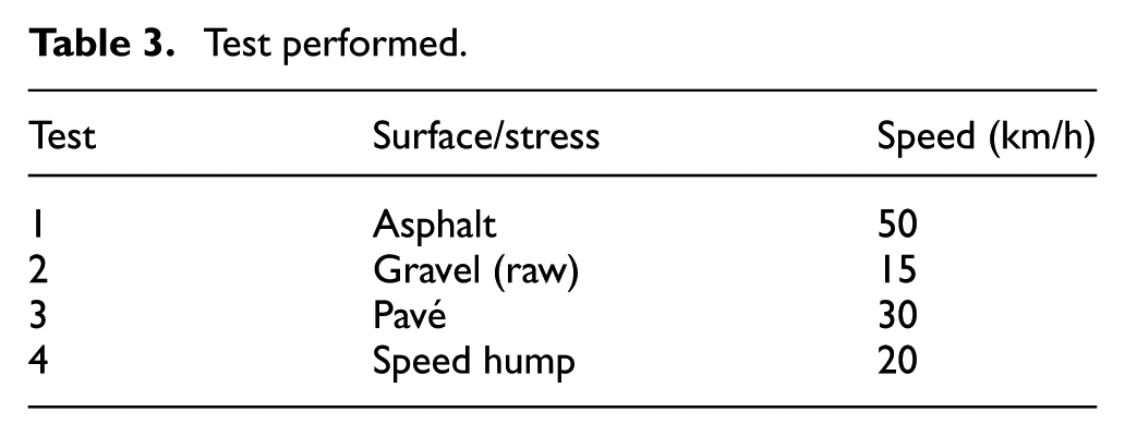
Several tests performed at constant speed on different road surfaces have been carried out to prove the effectiveness of the proposed method. Table 3 reports the complete list of tests performed while Figure 6 shows the surfaces and Figure 7 reports FFT plots for each surface.

Table 3.

Test performed.

Test	Surface/stress	Speed (km/h)
1	Asphalt	50
2	Gravel (raw)	15
3	Pavé	30
4	Speed hump	20

Figure 6.

Proving surfaces – 1: asphalt; 2: gravel; 3: pave; 4: speed hump.

Figure 7.

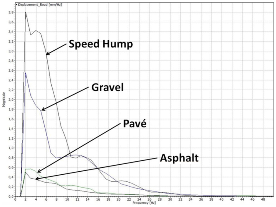
FFT plot for each surface.

The choice of different road surfaces at different speeds comes from the necessity to test the effectiveness of the road reproduction process for various levels of road energy input and in a reasonably wide target frequency range. The test vehicle was a standard BMW 3-series, MY 2010 (E91).

Results and discussion

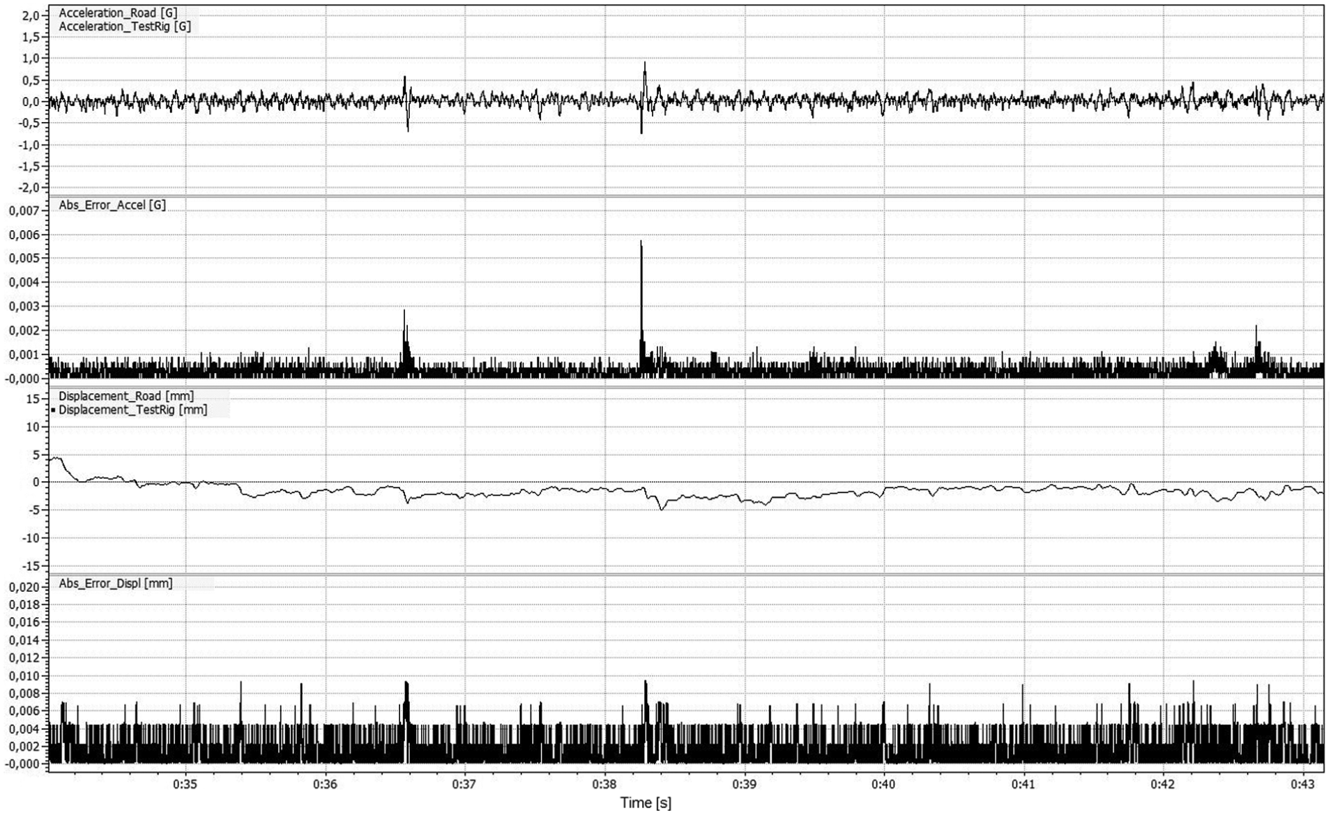
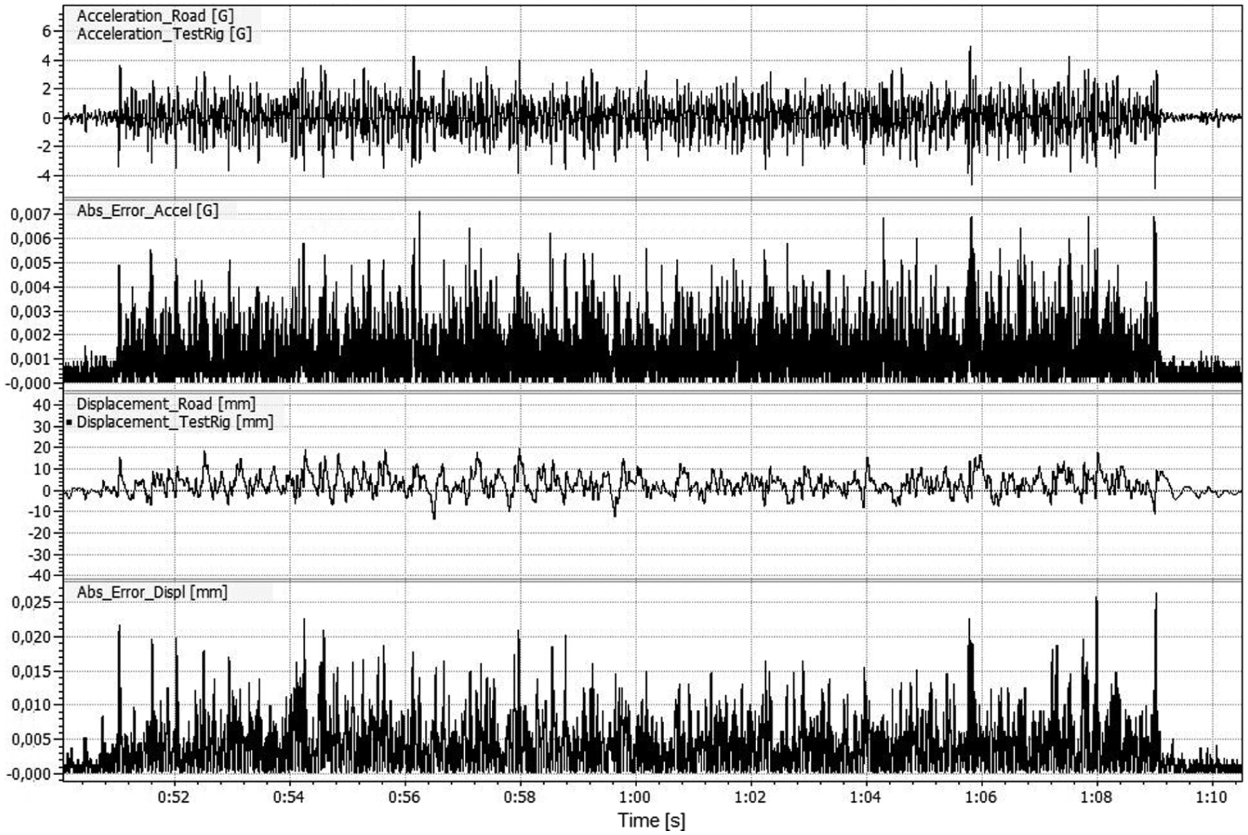
For the sake of brevity only, the front left corner will be considered in this section. In any case, the system performance is comparable on all four corners. Figures 7 –10 report comparisons between real-world and rig-generated road profile displacement data. It is worth to highlight that the difference between time histories of road and rig profiles is not visible when overlapping the two data streams because the system performance is very good. Therefore, the absolute error has been reported for each sensor as well. Also, RMS errors have been reported in Table 4 for completeness.

Figure 8.

Test on asphalt surface at 50 km/h constant.

Figure 9.

Test on gravel surface at 15 km/h constant.

Figure 10.

Test performed on paved surface at 30 km/h constant.

Table 4.

Errors summary.

Test	Acceleration MAE	Displacement MAE	Acceleration RMS	Displacement RMS
1	0.32%	0.25%	0.18%	0.16%
2	0.57%	0.66%	0.18%	0.20%
3	0.44%	0.48%	0.19%	0.23%
4	0.95%	0.98%	0.35%	0.33%

MAE: maximum absolute error; RMS: root mean square.

The test performed on good quality (smooth) road pavement at 50 km/h is reported in Figure 8. It shows very low acceleration and displacement levels. Under these conditions, the system can replicate road data very well, the maximum absolute error (MAE) being 0.32% for unsprung mass acceleration and 0.25% for displacement.

Figure 9 shows the test performed on an off-road gravel surface. In this case, amplitudes are higher as expected and many other frequencies come into play. Under these conditions, errors are slightly higher but still very low.

Results of the test carried out on the paved surface are shown in Figure 10. In this case, inputs coming from the road are lower in terms of amplitude to those of Figure 8 but at higher frequencies. Errors are still well under 1%.

Finally, in Figure 11, results of the test performed on a speed hump are shown. Data represent something very similar to an impulse, under this condition the worst reproduction performance occurs: acceleration MAE is 0.95% while displacement MAE is 0.98%. Table 4 summarizes the errors for each single road reproduction test.

Figure 11.

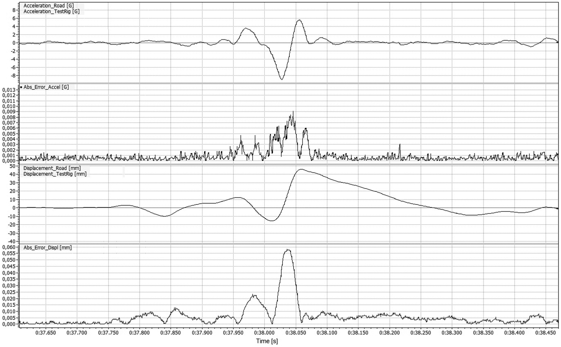
Test performed on a speed hump at 20 km/h constant.

Conclusion

In this article, a method to record and reproduce road profiles and vertical inputs on an indoor test rig has been presented. The road surface acquisition method is effective but also very cheap because only two common transducers per corner are required: a single axis accelerometer and a potentiometer. The test rig hardware is very simple as well and the MATLAB^®-based iterative control system has been proven to be fully reliable. Servo hydraulic control loop is very easy to set up and tune since it is based on a closed-loop PID controller which acts only on the actuator’s displacement, resulting in a more time-saving procedure.

Validation has been provided comparing real-world data and test rig data; results show that maximum errors are around 1% during every test, even during special surfaces reproduction such as speed humps. Moreover, a correlation between the error and the energy contribution of the surface to be reproduced (see Figure 7) can be seen. The higher is the energy contribution of the road surface, the higher will be the error.

Footnotes

Academic Editor: Francesco Massi

Declaration of conflicting interests

The author(s) declared no potential conflicts of interest with respect to the research, authorship, and/or publication of this article.

Funding

The author(s) received no financial support for the research, authorship, and/or publication of this article.

References

Makoto

Bayesian analysis for the results of fatigue test using full-scale models to obtain the accurate failure probabilities of the Shinkansen vehicle axle. Reliab Eng Syst Safe 2002; 75: 321–332.

Shafiullah

AKM

. Generation and validation of loading profiles for highly accelerated durability tests of ground vehicle components. Eng Fail Anal 2013; 33: 1–16.

Uberti

Gadola

Chindamo

et al . Design of a double wishbone front suspension for an orchard/vineyard tractor: a kinematic analysis. J Terramechanics 2015; 57: 23–39.

Benini

Gadola

Chindamo

et al . The influence of suspension component friction on race car vertical dynamics. Vehicle Syst Dyn 2016; 55: 1–13.

Marchesin

Gadola

Benini

et al . Upright mounted pushrod: the effects on racecar handling dynamics. In: Proceedings of the 24th international symposium on dynamics of vehicles on roads and tracks, Graz, Austria, 17–21 August 2015. Taylor & Francis.

Jayasurya

HPW

Sangpradit

. Dynamic performance and ride comfort evaluation of the seat suspension system in a small agricultural tractor to attenuate low-frequency vibration transmission. Agric Eng Int: CIGR J 2014; 16: 207–216.

Matthews

An analogue computer investigation of the potential improvement in tractor ride afforded by a flexible front axle. J Agric Eng Res 1967; 12: 48–54.

Rill

Salg

Wilks

. Improvement of dynamic wheel loads and ride quality of heavy agricultural tractors by suspending front axles. In: Proceedings of the 3rd international symposium on heavy vehicle weights and dimensions, Queens College, Cambridge, 28 June–2 July 1992. London: ICE Virtual Library.

Kharul

Balakrishnan

Karedla

et al . Virtual testing and correlation for a motorcycle design. SAE Int J Mater Manuf 2010; 3: 541–549.

10.

Uberti

Gadola

. Design of a new high-end street bike. In: 11th international design conference, DESIGN 2010, Dubrovnik, 17–20 May 2010, pp.1741–1752. Bristol: Design Society Administration.

11.

Tuluie

Ericksen

GS.

Racing motorcycle design process using physical and virtual testing methods (SAE technical paper). In: Motorsports engineering conference and exposition, Dearborn, MI, 13–16 November 2000. Warrendale, PA: SAE.

12.

Spickenreuther

Bersiner

Fricke

. Realistic driving experience of new vehicle concepts on the BMW ride simulator. SAE technical paper 2012-01-1548, 2012.

13.

Cambiaghi

Gadola

Vetturi

. Suspension system testing and tuning with the use of a four-post rig. In: Motorsports engineering conference and exposition, Dearborn, MI, 16–19 November 1998. Warrendale, PA: SAE.

14.

Vanhees

Maes

. Vehicle suspension characterisation by using road simulation on a 4 poster test rig. In: Proceedings of the 2002 international conference on noise and vibration engineering, ISMA, Leuven, 16–18 September 2002. Leuven: KU Leuven.

15.

Ibicek

Thite

AN.

In situ measurement of discomfort curves for seated subjects in a car on the four-post rig. Adv Acoust Vib 2014; 2014: Article 239178.

16.

Ibicek

Thite

AN.

Quantification of human discomfort in a vehicle using a four-post rig excitation. J Low Freq Noise V A 2012; 31: 29–42.

17.

Karajagikar

Rajhans

Ahuja

et al . Vibration analysis on driver seat for small cars (SAE technical papers). In: Symposium on international automotive technology, SIAT 2011, Pune, India, 19–22 January 2011. Warrendale, PA: SAE.

18.

Goktan

Yetkin

Road load data estimation on multiaxial test rigs for exhaust system vibrations (SAE technical paper). In: SAE 2002 world congress, Detroit, MI, 4–7 March 2002. Warrendale, PA: SAE.

19.

Czop

SŁawik

A high-frequency first-principle model of a shock absorber and servo-hydraulic tester. Mech Syst Signal Pr 2011; 25: 1937–1955.

20.

Cryer

Nawrocki

Lund

RA.

Road simulation system for heavy duty vehicles. SAE technical paper 760361, 1976.

21.

Dursun

Bayram

Tracking control solution for road simulators: model-based iterative learning control approach improved by time-domain modelling. Gazi Univ J Sci 2012; 25: 435–446.

22.

Plummer

AR.

Control techniques for structural testing: a review. Proc IMechE, Part I: J Systems and Control Engineering 2007; 221: 139–169.

23.

Hay

Roberts

DE.

Iterative control in automotive testing. Proc IMechE, Part I: J Systems and Control Engineering 2007; 221: 223–233.

24.

Dodds

Plummer

Laboratory road simulation for full vehicle testing: a review. SAE technical paper 2001-26-0047, 2001. DOI: 10.4271/2001-26-0047.

25.

Chen

J-Y

Wang

H-D

Zhou

J-C

et al . Progress in multi-exciter vibration testing control technology. J Vib Shock 2011; 30: 69–73.

26.

Gizatullin

Edge

KA.

Adaptive control for a multi-axis hydraulic test rig. Proc IMechE, Part I: J Systems and Control Engineering 2007; 221: 183–198.

Reproduction of real-world road profiles on a four-poster rig for indoor vehicle chassis and suspension durability testing

Abstract

Keywords

Introduction

The test rig

Materials and method

Control system hardware setup

Software configuration

System model

Set of sensors

Road profiles and test vehicle

Results and discussion

Conclusion

Footnotes

Declaration of conflicting interests

Funding

References