Sage Journals: Discover world-class research

Abstract

In this article, we propose a fast method to solve large-scale three-dimensional topology optimization problems subject to buckling constraints. Buckling analysis entails the solution of a generalized eigenvalue problem. For problems with large degrees of freedom, the current numerical methods tend to be memory-hungry, leading to high computational costs. First, a low-memory assembly-free linear buckling analysis method is proposed. Specifically, this method is based on the voxelization model, an assembly-free version of the deflated conjugate gradient is used to accelerate the iteration solution of linear systems of equations, where neither the stiffness matrix nor the deflation matrix is assembled, and the parallelization of matrix–vector multiplication is achieved by the congruency of voxels. Due to the particularity of the stress stiffness matrix in the buckling analysis, the inverse iteration is used to solve the general eigenvalue problem, which can reduce the operations of stress stiffness matrix considerably. Based on the efficient buckling analysis method, we extend the level-set method for buckling constraints in a semi-analytical manner. Several numerical experiments demonstrate that the proposed method can solve large-scale three-dimensional buckling analysis and topology optimization against buckling constraints effectively.

Keywords

Topology optimization buckling assembly-free finite element analysis

Introduction

Buckling is the sudden failure of a structural member to carry compressive load.¹ Buckling analysis has important applications in aerospace, civil engineering, mechanical engineering, and other fields. Linear buckling analysis (also known as eigenvalue buckling analyses) is a classical engineering method for determining the buckling load of structures.^2,3 Linear buckling analysis is included in most finite element analysis (FEA) softwares today and can be applied to very large structural models with millions of elements, for example, the buckling behavior of complex composites structures is analyzed by Ansys.^4,5 But they tend to be memory-hungry, leading to high computational costs for problems with large degrees of freedom (DOFs). The high computational costs might be acceptable for buckling analysis but it will be exacerbated in applications in buckling-constrained topology optimization, where one must solve buckling problems repeatedly. This is one of the bottlenecks and restricts the development of buckling topology optimization: while the theory of topology optimization has reached a high level of maturity, large-scale three-dimensional (3D) optimization involving millions of DOF is one of the challenges that remain today, it can take hours, or even days to complete; FEA software like HyperWorks can only use two-dimensional (2D) elements with nonzero thickness for buckling-constrained topology optimization.

One of the established methods for solving the generalized buckling eigenvalue problem is the block Lanczos algorithm^6,7 that requires repeated solution of a linear system of equations where the matrix is a linear combination of K and K_σ that is determined dynamically. Since both K and K_σ are large, and since the linearly combined matrix is constantly changing, explicit factorization can be expensive. Alternative strategies use preconditioned iterative solver. However, these can be slow to converge, while accuracy is severely compromised with early termination.^6–8 Alternatively, computing an approximate inverse over Krylov sub-space has been proposed in previous studies.^6–8

Other algorithms for solving eigenvalue problem include “locally optimal block preconditioned conjugate gradient,”“Davidson-Jacobi,” and so on that have been demonstrated to be competitive for large-scale eigenvalue problem in Arbenz et al.⁶ One such algorithm is the subspace-augmented Rayleigh–Ritz conjugate gradient (RCG) that exploits the assembly-free aspect presented for solving linear systems.⁹ While RCG is efficient for large-scale modal analysis, as discussed in Suresh and Yadav,¹⁰ it cannot be applied here effectively for reasons described later in the next section.

In addition to finite element method (FEM) method, there are some other effective numerical methods that can be used for buckling analysis. Meshfree method is used for buckling analysis of Reissner–Mindlin plates by Bui et al.¹¹ Valizadeh et al.^12,13 studied the buckling of orthotropic plates and the thermal buckling of functionally graded material plates numerically by isogeometric analysis. Yu et al.¹⁴ utilize extended isogeometric analysis to solve the thermal buckling analysis of functionally graded plates with internal defects. Liu et al.¹⁵ analyzed buckling failure of cracked composite functionally graded plates by extended finite element method (XFEM).

Topology optimization is a systematic method of generating designs to meet specific engineering requirements. In many of these applications, buckling failure must be accounted for during topology optimization,¹⁶ leading to a buckling-constrained topology optimization problem. Different topology optimization methods have been proposed to solve such problems, including solid isotropic material with penalization (SIMP), evolutionary, and level-set.

SIMP uses pseudo-densities assigned to elements, and they vary between 0 and 1. These pseudo-densities are then used as continuous relaxation parameter.¹⁷ However, when continuous relaxation method is used in the context of buckling modes, undesirable numerical effects are observed;¹⁸ Pedersen¹⁹ and Neves et al.²⁰ discuss the spurious modes computed in continuous relaxation method. They consider assigning zero stiffness to such elements to overcome these issues, but this will result in inconsistencies in the model. The variability in densities from element to element also causes ill-conditioning of the stiffness matrices.^21,22 Additionally, for stress-related analysis, the accuracy over gray elements is poor.

As an alternative to SIMP, a free material optimization (FMO) was proposed in Browne et al.²³ FMO considers the entire stiffness tensor as a continuous design variable. The sensitivity computation for compliance and stress field becomes more expensive. A binary programming method is discussed in Allaire and Jouve,²⁴ where the bottleneck is in computing the derivatives of buckling constraints.

The other strategy for solving topology optimization relies on defining the evolving topology through a level-set.²⁵ Level-set allows the domain to be well defined at all times, thus overcoming the issue of ill-conditioned stiffness matrices. Numerous examples are provided in the literature to illustrate the effectiveness of the level-set–based methods.^26–28

In this article, a simple inverse iteration driven, assembly-free deflated conjugate gradient method for solving linear buckling problem is proposed. Then, we extend the level-set method for buckling-constraint topology optimization in a semi-analytical manner, and the buckling load sensitivity is computed in an adjoint method. Finally, numerical results are presented to illustrate the proposed method, followed by conclusions and open issues.

Assembly-free buckling analysis

The linear buckling behavior of a structure is governed by the following general eigenvalue problem

(K + λ_{i} K_{σ}) v_{i} = 0

(1)

where K is the global stiffness matrix that is sparse and positive definite; K_σ is called the global stress stiffness matrix or global geometric stiffness matrix; λ_i is the ith eigenvalue, and v_i is the corresponding eigenvector. In particular, the lowest eigenvalue λ₁ determines the buckling safety factor (SF),²⁹ that is, the critical load at which buckling will occur. The vector v₁ represents the corresponding buckling mode.

FEA of linear buckling is typically carried out in two stages. In the first stage, the structural member is subject to a unit load. A finite element mesh of the domain is constructed, and the corresponding static linear elasticity problem is posed and solved, which equivalents to solving a linear system of equations

K u = f

(2)

Here u is the global displacement vector, and f is the global load vector. In the second stage, the linear displacement field u is post-processed to obtain the stress tensor within each of the element.²⁹ Then the stress tensor is used to define an element-level stress stiffness matrix K_σ^e. This is then assembled to construct the global stress stiffness matrix K_σ. Finally, the generalized eigenvalue problem (1) is solved.

In the present article, an accelerated buckling FEA is developed by implementing and merging three distinct but complementary concepts: voxelization, assembly-free deflation, and inverse iteration. Based on the above infrastructure, fine-grained parallelization is achieved in this article on multi-core CPUs using OpenMP.

Voxelization

Voxelization is a special form of spatial discretization where the geometry is approximated via uniform hexahedral elements or “voxels.” The voxelization process is straightforward and is discussed in Hughes et al.³⁰ The most important benefits of voxelization are meshing-robustness and low memory footprint, especially in combination with assembly-free analysis. This ensures a faster sparse matrix-vector multiplication (SpMV) through parallel implementation on multi-core architectures. The voxelization of a complex geometry is illustrated in Figure 1; it has over 300,000 elements. Fortunately, even such a large-sized problem is easily handled via the proposed method.

Figure 1.

Voxelization of rocker.

Assembly-free deflation for static analysis

Assembly-free FEA was proposed by Hughes and others in 1983,³¹ but has resurfaced due to the surge in fine-grained parallelization. The basic concept here is that the stiffness matrix is never assembled; instead, the fundamental matrix operations such as the SpMV are performed in an assembly-free elemental level as

K v = \underset{a s s e m b l e}{Π} (K_{e} v_{e})

(3)

Assembly-free SpMV is particularly advantageous if memory footprint can be reduced by storing limited data. Exploiting element congruency helps reduce memory footprint.⁹ Second, assembly-free iterative analysis is effective only if an assembly-free acceleration/preconditioning can be exploited; here, we rely on assembly-free deflation.

Deflation is a powerful acceleration technique for conjugate gradient³² and is more amenable to an assembly-free implementation than classic preconditioners such as incomplete Cholesky. The particular method of deflation exploited in this article is based on rigid-body agglomeration discussed in Ipsen³³ The rigid-body agglomeration has a simple assembly-free implementation and offers significant advantage in parallel computing.⁹

The first step in assembly-free buckling analysis (AFBA) is solving equation (2). This is accomplished here using the deflated conjugate gradient method discussed in Yadav and Suresh.⁹ Deflated conjugate gradient uses several different agglomeration groups to accelerate the solver. The solution of equation (2) generates the displacement and stress fields.

Inverse iteration for buckling analysis

As discussed in the literature review, the generalized eigenvalue problem for buckling is similar to modal analysis. Therefore, based on the earlier work,¹⁰ we attempted to use RCG algorithm that requires repeated operations Kv and K_σv. Unfortunately, RCG is efficient only if we can exploit congruency and limit the number of unique elements for both operations. In the case of stiffness matrix K, one can certainly exploit the congruency in the voxel mesh. However, for buckling analysis, each element stress stiffness matrix depends on its own stress tensor, which makes the advantage of congruency cannot be utilized. Furthermore, storing every element stress stiffness matrix K_σ will create a large memory footprint and slow down the computation.

This draws attention toward another method known as inverse iteration.³⁴ The basic principle is to carry out

y = - K^{- 1} K_{σ} v

(4)

and to use the solution repeatedly. The number of K_σv operations is considerably reduced, and the computational burden falls on solving an equivalent static problem.⁹

The algorithm of using inverse iteration to solve equation (5) is described as follows:

Initialize v⁽¹⁾ ≠ 0 such that ||v⁽¹⁾|| = 1

Set i = 1

Compute z⁽ⁱ⁾ = K_σv⁽ⁱ⁾

Solve Ky⁽ⁱ ⁺ ¹⁾ = z⁽ⁱ⁾ for y⁽ⁱ ⁺ ¹⁾

Update v⁽ⁱ ⁺ ¹⁾ = y⁽ⁱ ⁺ ¹⁾/||y⁽ⁱ ⁺ ¹⁾||

Compute g⁽ⁱ⁾ = Kv⁽ⁱ ⁺ ¹⁾ + K_σv⁽ⁱ ⁺ ¹⁾

If ||g⁽ⁱ⁾|| ≤ε, terminate; else, increase i, and go to Step 3

Once the algorithm converges to a mode shape v, the eigenvalue can be computed through

λ = \frac{v^{T} K v}{v^{T} K_{σ} v}

(5)

The number of iterations required to converge to the mode shape is far smaller than RCG as the numerical error is primarily eliminated in the linear solution in Step 4. The numerical results illustrate the advantage of using assembly-free inverse iteration with deflated conjugate gradient for buckling analysis. An efficient buckling analysis creates an opportunity to apply buckling constraints during topology optimization. We discuss the formulation in the next section.

Topology optimization

Buckling load factor sensitivity

The element sensitivity is the expected change in buckling load factor when an element is deleted from the mesh. We use discrete variable $x_{e}$ , where $x_{e}$ represents whether an element e is present or not. This can be represented as

\frac{d λ}{d x_{e}} = - \frac{v^{T} (\frac{d K}{d x_{e}} + λ \frac{d K_{σ}}{d x_{e}}) v}{v^{T} K_{σ} v}

(6)

Calculating the sensitivities of the buckling load is rather tedious. It seems that the similarity to eigenfrequency optimization can be used. However, in contrast to the mass matrix sensitivity for eigenfrequency analysis, the stress stiffness sensitivity $d K_{σ} / d x_{e}$ is not readily available.

The stress stiffness matrix is an implicit function of the displacement field. That is

K_{σ} = K_{σ} (u (x_{e}), x_{e})

(7)

Then the total derivative of the stress stiffness matrix is

\frac{d K_{σ}}{d x_{e}} = \frac{\partial K_{σ}}{\partial x_{e}} + \frac{\partial K_{σ}}{\partial u} \frac{d u}{d x_{e}}

(8)

For the second term on the right-hand side of equation (8), we have

\frac{\partial K_{σ}}{\partial u} \frac{d u}{d x_{e}} = \sum_{d o f = 1}^{N} (\frac{\partial K_{σ}}{\partial u_{1}} \frac{d u_{1}}{d x_{e}} + \frac{\partial K_{σ}}{\partial u_{2}} \frac{d u_{2}}{d x_{e}} + \dots + \frac{\partial K_{σ}}{\partial u_{N}} \frac{d u_{N}}{d x_{e}})

(9)

In order to get the full derivative of displacement u_i, we start from the static equilibrium equation (2). Differentiate equation (2) with respect to the design variable x_e

K \frac{du}{d x_{e}} + \frac{d K}{d x_{e}} u = \frac{d f}{d x_{e}}

(10)

Since the design-dependent force is not considered and the external loads are independent on x_e, we have

\frac{d f}{d x_{e}} = 0

(11)

\frac{d u}{d x_{e}} = K^{- 1} (- \frac{\partial K}{\partial x_{e}} u) = K^{- 1} {[\begin{matrix} 0 & 0 & 0 \\ 0 & k^{e} & 0 \\ 0 & 0 & 0 \end{matrix}]}_{NXN} u_{NX 1}

(12)

The left-hand side of above equation is of dimension N × 1. Then the term $d u_{i} / d x_{e}$ in equation (9) is the ith term. Now, in order to get the $\partial K_{σ} / \partial u_{i}$ on the right-hand side in equation (9), we have

\frac{\partial K_{σ}}{\partial u_{i}} = Π_{a s s e m b l e}^{4 e l e m s} \frac{\partial K_{σ}^{e}}{\partial u_{i}}

(13)

where four elements represent four surrounding elements around one specific node with perturbed displacement u_i.

For one of the four elements, each stress tensor in stress stiffness matrix is the first-order function of u_i, and then, we can explicitly write out

\frac{\partial {K_{σ}}^{e}}{\partial u_{i}} = \int G^{T} [\begin{matrix} \frac{\partial S^{e}}{\partial u_{i}} \\ \frac{\partial S^{e}}{\partial u_{i}} \\ \frac{\partial S^{e}}{\partial u_{i}} \end{matrix}] G d V

(14)

where G is obtained from shape functions [N] by appropriate differentiation and ordering of terms

[G] = [\begin{matrix} \frac{\partial N_{1}}{\partial x} & 0 & 0 & \frac{\partial N_{2}}{\partial x} & 0 & 0 & \dots & \frac{\partial N_{8}}{\partial x} & 0 & 0 \\ \frac{\partial N_{1}}{\partial y} & 0 & 0 & \frac{\partial N_{2}}{\partial y} & 0 & 0 & \dots & \frac{\partial N_{8}}{\partial y} & 0 & 0 \\ \frac{\partial N_{1}}{\partial z} & 0 & 0 & \frac{\partial N_{2}}{\partial z} & 0 & 0 & \dots & \frac{\partial N_{8}}{\partial z} & 0 & 0 \\ 0 & \frac{\partial N_{1}}{\partial x} & 0 & 0 & \frac{\partial N_{2}}{\partial x} & 0 & \dots & 0 & \frac{\partial N_{8}}{\partial x} & 0 \\ 0 & \frac{\partial N_{1}}{\partial y} & 0 & 0 & \frac{\partial N_{2}}{\partial y} & 0 & \dots & 0 & \frac{\partial N_{8}}{\partial y} & 0 \\ 0 & \frac{\partial N_{1}}{\partial z} & 0 & 0 & \frac{\partial N_{2}}{\partial z} & 0 & \dots & 0 & \frac{\partial N_{8}}{\partial z} & 0 \\ 0 & 0 & \frac{\partial N_{1}}{\partial x} & 0 & 0 & \frac{\partial N_{2}}{\partial x} & \dots & 0 & 0 & \frac{\partial N_{8}}{\partial x} \\ 0 & 0 & \frac{\partial N_{1}}{\partial y} & 0 & 0 & \frac{\partial N_{2}}{\partial y} & \dots & 0 & 0 & \frac{\partial N_{8}}{\partial y} \\ 0 & 0 & \frac{\partial N_{1}}{\partial z} & 0 & 0 & \frac{\partial N_{2}}{\partial z} & \dots & 0 & 0 & \frac{\partial N_{8}}{\partial z} \end{matrix}]

(15)

\frac{\partial S^{e}}{\partial u_{i}} = [\begin{matrix} \frac{\partial σ_{x}}{\partial u_{i}} & \frac{\partial τ_{x y}}{\partial u_{i}} & \frac{\partial τ_{x z}}{\partial u_{i}} \\ \frac{\partial τ_{x y}}{\partial u_{i}} & \frac{\partial σ_{y}}{\partial u_{i}} & \frac{\partial τ_{y z}}{\partial u_{i}} \\ \frac{\partial τ_{xz}}{\partial u_{i}} & \frac{\partial τ_{yz}}{\partial u_{i}} & \frac{\partial σ_{z}}{\partial u_{i}} \end{matrix}]

(16)

It is noted that those K_σ^e should be mapped back to N × N global matrix. Now equation (6) can be written as

\frac{d λ}{d x_{e}} = \frac{- v^{T} \frac{dK}{d x_{e}} v - λ v^{T} \frac{\partial K_{σ}}{\partial x_{e}} v - λ v^{T} \frac{\partial K_{σ}}{\partial u} \frac{du}{d x_{e}} v}{v^{T} K_{σ} v}

(17)

For the sensitivity of each element, the inverse global stiffness matrix is involved. In order to get one complete sensitivity field, equation (12) needs to be solved for m times (m is the number of elements); this is not suitable for topology optimization, as the computation time increases exponentially with the number of design variables, and the sensitivity fields need to be computed many times during the topology optimization.

A better way to compute the sensitivities of the buckling load is by adding adjoint variables and constraint functions. By choosing the adjoint variables correctly, it is possible to replace the complicated parts of the sensitivity equation by expressions that are easier to calculate. In order to get the sensitivity with respect to λ, we add the adjoint term µ

v^{T} (K + λ K_{σ}) v + μ^{T} [K u - f] = 0

(18)

where the adjoint µ links the deformation to external force.

Then, take derivative of equation (18), we get

\begin{matrix} 2 {\frac{d v}{d x_{e}}}^{T} (K + λ K_{σ}) v + v^{T} (\frac{d K}{d x_{e}} + λ \frac{d K_{σ}}{d x_{e}} + \frac{d λ}{d x_{e}} K_{σ}) v \\ + μ^{T} (\frac{d K}{d x_{e}} u + K \frac{d u}{d x_{e}} - \frac{d f}{d x_{e}}) = 0 \end{matrix}

(19)

Since equation (1), the first term in equation (19) is equal to 0. Now the adjoint µ is chosen such that $du / d x_{e}$ is dropped from the equation, that is

v^{T} λ \frac{\partial K_{σ}}{\partial u} \frac{d u}{d x_{e}} v + μ^{T} (K \frac{d u}{d x_{e}}) = 0

(20)

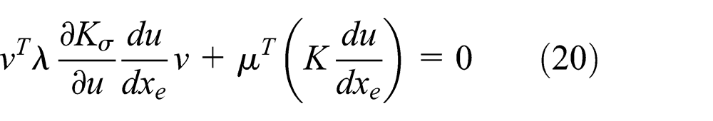
After factoring out and rearranging, we have

K μ = - λ (v^{T} \frac{\partial K_{σ}}{\partial u} v)

(21)

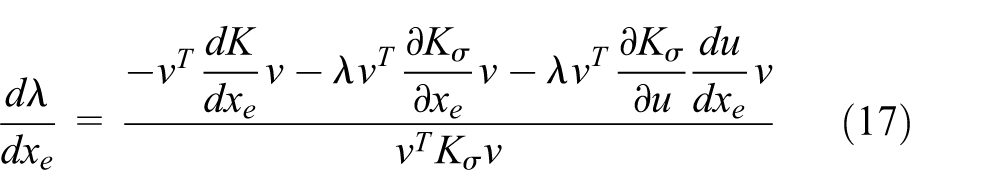
where the calculation of $\partial K_{σ} / \partial u$ is same as equations (13), (14), and (16); µ is the adjoint displacement, which can be solved by assembly-free deflated conjugate gradient in the previous section.

Then, equation (19) can be simplified as

v^{T} (\frac{d K}{d x_{e}} + \frac{d λ}{d x_{e}} K_{σ} + \frac{\partial K_{σ}}{\partial x_{e}}) v + μ^{T} (\frac{d K}{d x_{e}} u) = 0

(22)

Thus, the sensitivity can be shown as

\frac{d λ}{d x_{e}} = \frac{- v^{T} Δ K^{e} v - v^{T} Δ {K_{σ}}^{e} v - μ^{T} Δ K^{e} u}{v^{T} K_{σ} v}

(23)

To get a complete sensitivity field, equation (21) only need to be solved once, which makes the adjoint method much faster.

Level-set

A straightforward approach to exploit element sensitivity is to use the information to delete elements with lower sensitivity values. However, this method would lead to same issues of creating checker board pattern and instability in the mesh. However, sensitivity field can be used as a level-set³⁵ that traces the Pareto curve governing compliance and volume fractions. The Pareto-optimal designs can result in better conditioned stiffness matrices, and consequently faster iterative convergence. The objective of this article is to generalize this to buckling-constrained topology optimization problem.

Given the sensitivity field T and a cutting manifold corresponding to a cut-off value τ, one can define a domain $Ω^{τ}$ according to

Ω^{τ} = {e | T (e) > τ}

(24)

This will determine the set of points with sensitivity values greater than an arbitrary value of τ. The sensitivity field provides a direct “pseudo-optimal” domain for a specific volume reduction that can be determined by cutting manifold. The computed domain, however, may not be optimal,³⁵ that is, it may not be the best possible design for objective function with given volume fraction. Reducing the volume fraction may change the sensitivity field, and therefore, one must repeat the following steps: (1) solve the finite element problem over $Ω$ , (2) re-compute the sensitivity field, and (3) reset the cutting manifold for desired volume fraction.

Once convergence has been achieved for the desired volume fraction, one can move forward with the next step of volume reduction, repeating the above process.

Algorithm

A buckling-constrained topology optimization problem must account for buckling failure during topology optimization

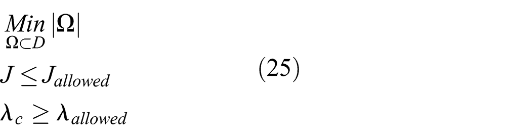
\begin{matrix} \underset{Ω \subset D}{M i n} | Ω | \\ J \leq J_{a l l o w e d} \\ λ_{c} \geq λ_{a l l o w e d} \end{matrix}

(25)

where Ω is the domain of objective topology, D is the allowable design space, J is the compliance of structure, J_allowed is the maximum allowable compliance, λ_c is the critical buckling load, and λ_allowed is the minimum allowable critical buckling load

Typically, the sensitivity field T is well defined for an unconstrained problem. When constraints are involved, the sensitivity field of the objective (compliance) must be combined with those of the constraints (in this case, buckling) through weighting factors. The weighting factors are determined along the lines described in Yang and Chen³⁷ The concept of weighting functions was explored in SIMP-based implantation.³⁷Furthermore, in Ref.,³⁶ it was determined through numerical experiments that a quadratic function g is more reliable and efficient. Based on these results, we adopt the following weighting

T_{w} = T_{J} + {(\frac{λ_{a l l o w e d}}{λ})}^{2} T_{b}

(26)

$T_{w}$ is the weighted sensitivity field, $T_{J}$ is the sensitivity field of compliance, and $T_{b}$ is the sensitivity field of critical buckling load.

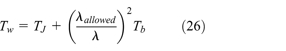
In other words, if the current buckling load factor is much greater than the minimum allowed, then less weightage is applied on the corresponding sensitivity field. By controlling the allowable critical buckling load, we show that a dynamic tradeoff can be maintained. The complete algorithm is described in the following:

The allowable domain is initialized and discretized.

The initial FEA requires a static solve and a buckling modal analysis by solving equations (1) and (2). Hence, FEA would refer to solving both equations.

Based on the FEA, sensitivity field for the objective (compliance) and buckling is computed. Based on proximity to imposed constraints, weight parameters (multipliers) are computed as described in Yang and Chen.³⁷

The desired volume fraction is used to determine the cutting manifold.

If the relative compliance change is smaller than 1%, it is assumed that the process step converged and then we go on to Step 6. If the parameter has not yet converged, a smaller volume fraction decrement Δv is used and we go to Step 8.

FEA is used to compute the constraint parameter.

If constraints are met, we return to Step 3 and repeat the process. Else, the volume fraction decrement Δv is reduced and we go to Step 8.

If the volume fraction decrement is too small, the algorithm terminates, else algorithm returns to Step 4. For the numerical examples at the next section, the volume fraction decrement Δv is initialized to 0.05, and Δv_min is set to 0.0025.

Figure 2 illustrates the algorithm described above.

Figure 2.

Proposed algorithm.

Numerical results

In this section, we compare the results of buckling analysis using the proposed method, against those obtained through SolidWorks. The material properties for all examples are those of steel with E = 2.1 × 10¹¹ Pa and υ = 0.33.

Buckling of a rectangle beam

The first example is that of a beam of 1 m in length, and 100 mm by 10 mm cross-section. The beam is fixed at one end, and a compressive unit load is applied at the other. The classic fixed-free Euler-beam analysis yields a critical load of

P_{c r} = \frac{π^{2} E I}{{(2 L)}^{2}} = 4314

(27)

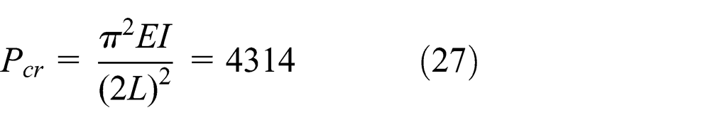
The results obtained through the proposed AFBA and those obtained from SolidWorks and Hyperworks using the same number of DOFs are illustrated in Figure 3. Both AFBA and SolidWorks methods converge to a critical load of 4344 N; the critical load got from Hyperworks is 4372 N. Note that we do not expect 3D FEA results to converge to the exact Euler-buckling result in equation (27); however, we do expect similar results.

Figure 3.

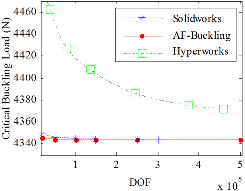
Predicted critical load using proposed AFBA, SolidWorks, and Hyperworks.

The real advantage of AFBA is in speed. Figure 4 illustrates the computing time for AFBA versus SolidWorks and Hyperworks. The quadratic growth in computation in SolidWorks and Hyperworks can be attributed to the quadratic growth in memory consumption with increasing DOFs.

Figure 4.

Computing time for AFBA, SolidWorks, and Hyperworks.

Buckling analysis of cylindrical column

To illustrate the potential deficiency of AFBA, we consider an example of a circular cylinder of 1 m in length and a radius of 10 mm. The classic fixed-free Euler-beam analysis yields a critical load of

P_{c r} = \frac{π^{2} E I}{{(2 L)}^{2}} = 4063

(28)

The predicted buckling loads are illustrated in Figure 5. AFBA method converges to a critical load of 4195 N, SolidWorks is 4081 N, and Hyperworks is 4041 N. The difference can be attributed to the voxelization in AFBA. Local stress variation in the voxelized meshes is an issue that will be addressed in the future.

Figure 5.

Accuracy plot for cylindrical column.

However, for topology optimization, the relative magnitudes of the sensitivities is more important than the accuracy. Furthermore, in topology optimization, the domain must necessarily be discretized using a large number of elements, and thus, speed becomes an important issue.

The time taken to solve the problem follows a similar trend as illustrated in Figure 6. Thus, if one can tolerate a few percent error, the voxelized AFBA method can be significantly faster.

Figure 6.

Computing time versus DOF for cylindrical column.

Buckling analysis of an L-shaped plate

Figure 7 shows an L-shaped plate and its dimensions. The thickness of the plate is 2 mm. The top of the plate is clamped, and a unit upward force is added on the left edge.

Figure 7.

L-shaped plate.

The results for the critical buckling load computed with 300,000 DOF are show in Table 1. The error in the solution is 0.5%. Since the computing time is related to the DOF of the model, the time comparison of this example is similar to that of the first two examples. With the increase of the DOF of the model, this proposed method shows the obvious advantage of the computing speed.

Table 1.

Predicted critical buckling load for L-shaped plate.

	Critical buckling load (N)	Time (s)
SolidWorks	1331.1	623
Hyperworks	1328.4	310
AF-Buckling	1334.6	30

Buckling analysis of a curved plate

In this example, we consider a curved plate under compression load as shown in Figure 8. The dimensions of the plate are 100 × 100 × 3 mm, and the radius of curvature is 100 mm.

Figure 8.

Curved plate.

The results for the critical buckling load computed with 400,000 DOFs are shown in Table 2. Here, we observe a 2.3% error in the solution. The proposed method utilized the voxelization; the downside of voxelization is that the stresses tend to be less accurate, since the voxelization cannot conform to the geometry completely, especially for rounded and curved structures. Linear buckling analysis is based on the linear elasticity theory of small displacement and small strain. The critical buckling load predicted by linear buckling analysis is not precise, which is usually higher than the actual value, especially for plate and shell. Usually, the linear buckling analysis is not used to get the precise buckling load, but used to get an approximate value quickly for the nonlinear buckling analysis. In this case, the speed is more important than accuracy; thus, if one can tolerate a few percent errors, the voxelized AFBA method can be significantly faster.

Table 2.

Predicted critical buckling load for curved plate.

	Critical buckling load (N)	Time (s)
SolidWorks	1.076 × 10⁵	1250
Hyperworks	1.089 × 10⁵	828
AF-Buckling	1.101 × 10⁵	47

Optimizing a thin column

We now consider minimizing the volume of a thin column with compressive load, as illustrated in Figure 9. Specifically, the objective is to solve the topology optimization problem

\begin{matrix} \underset{Ω \subset D}{M i n} | Ω | \\ J \leq 5 J_{0} \\ λ_{c} L_{0} \geq (SF) L_{0} \end{matrix}

(29)

Figure 9.

Thin column with compressive load.

In other words, the maximum allowable compliance J is five times its initial value J₀. For the buckling constraint, a SF was prescribed with respect to the initial load L₀, and the critical buckling load factor λ_c must be greater than the SF.

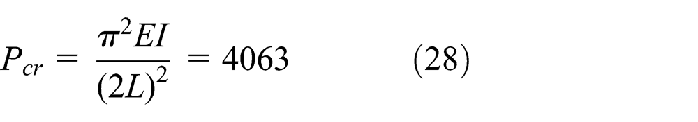
The structure was voxelized with 500,000 DOF, and the time taken for buckling analysis was 46 s. As the SF is increased in equation (29), the buckling constraint begins to dominate, resulting in topologies illustrated in Figure 10.

Figure 10.

Stiff designs with different safety factors: (a) no buckling constraint, (b) SF = 1.1, (c) SF = 1.5, and (d) SF = 2.

Furthermore, as the SF is increased, the optimization terminates at a higher volume fraction (see Table 3), as expected.

Table 3.

Minimizing volume for stiff structure.

Prescribed SF	Final volume fraction	Time (min)	#FEA
No constraint	0.3	15	64
1.1	0.3	38	86
1.5	0.42	42	98
2	0.52	24	74

SF: safety factor; FEA: finite element analysis.

Clutch rest pedal

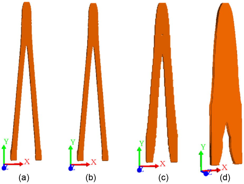
We now consider some practical problems. Figure 11 shows a pedal box of a high-performance vehicle; the weights of the parts on this vehicle must be reduced as much as possible. The left side of the pedal box is a clutch rest pedal.

Figure 11.

(a) Pedal box, (b) stress field, and (c) buckling mode.

The design requirement is to withstand the maximum load of 700 N. The FEA analysis result is shown in Figure 11(b) and (c). After the FEA analysis, the maximum stress is 398 MPa. As the material is high-strength aluminum alloy, and the yield strength is 435 MPa, the original design appears to meet the strength requirement. However, after the buckling analysis through the proposed AFBA method, the critical buckling load is 634 N, which means that when the maximum load is added, the pedal will fail because of buckling.

So the pedal needs to be optimized under the buckling constraint. The initial design domain is shown in Figure 12(a), and its volume is V₀. The original design on Figure 11 is 87% of V₀. The maximum allowable compliance is five times the initial value, and the buckling constraint is set as 700 N. The topology optimization problem is

\begin{matrix} \underset{Ω \subset D}{M i n} Ω \\ J \leq 5 J_{0} \\ λ_{c} \geq 700 N \end{matrix}

(30)

Figure 12.

Optimized with buckling constraint: (a) initial design domain and (b) optimized result.

The voxelized structure has 220,000 DOF, and the optimization time is 37 min. The optimized result is shown in Figure 12(b). The finial volume fraction of the result is 81%, which is smaller than the original design, but the critical buckling load is higher. Topology optimization can provide a conceptual design at the initial stage of the design. Topology optimization optimized the material distribution, which can be a reference for the further detailed design.

Camber link

Figure 13(a) shows a camber link of a multi-link suspension on the vehicle. The thickness of the upper edge is 20 mm, and the thickness of the lower rib is 5 mm. Buckling is one of the failure reasons of the camber link, and it needs to be considered carefully.

Figure 13.

(a) Camber link and (b) buckling mode.

First, the buckling analysis is performed by AFBA, as shown in Figure 13(b). The left hole is fixed, and a unit pressing force is added at the right hole. After the buckling analysis, the critical buckling load is 14,500 N, and the computing time is 29 s with 167,000 DOF. When the critical buckling load of 14,500 N is added to the camber link, the maximum stress is 419 MPa, which is lower than the yield strength (620 MPa). The camber link will fail because of buckling, as the buckling will happen before the yield. So the camber link needs a topology optimization for buckling problem.

The initial design domain is shown in Figure 14(a). The thickness of the camber link is increased to make more design space. The maximum allowable compliance is five times the initial values. The design requirement load is 20,000 N. The topology problem is

\begin{matrix} \underset{Ω \subset D}{M i n} Ω \\ J \leq 5 J_{0} \\ λ_{c} \geq 20, 000 N \end{matrix}

(31)

Figure 14.

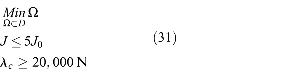
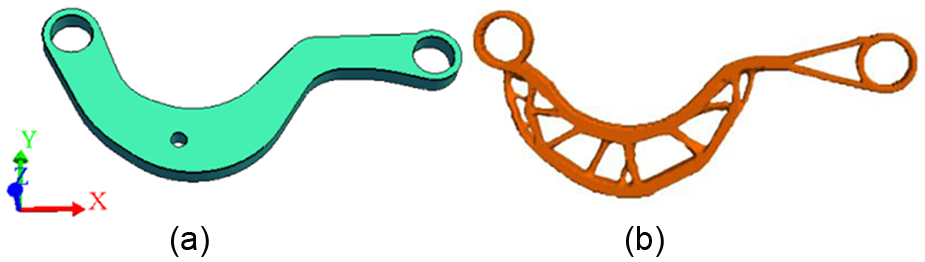
Optimized with buckling constraint: (a) initial design domain and (b) optimized result.

The optimized topology is shown in Figure 14(b). The voxelized structure has 350,000 DOF, and the optimization time is 27 min. The finial volume fraction is 50%, so the optimized structure is same weight as the original design but has a higher critical buckling load which can satisfy the practical design requirements.

Conclusion and future work

The main contribution of the article is an efficient method for large-scale buckling-constrained topology optimization problems. We propose an assembly-free method for linear buckling analysis by merging four distinct but complementary concepts: voxelization, assembly-free FEA, deflated conjugate gradient, and parallelization. In this method, the congruency of voxels is exploited to reduce the memory footprint and offers significant advantage in parallel computing, deflation is used to accelerate the iteration solution of linear systems of equations, and neither the stiffness matrix nor the deflation matrix is assembled. The resulting implementation is simple and well suited for parallelization. Combining the buckling analysis method with the level-set method, the topology optimization against buckling constraint can be solved efficiently. Future work will focus on post-buckling analysis that is critical for topology optimization.

Footnotes

Academic Editor: Jianqiao Ye

Declaration of conflicting interests

The author(s) declared no potential conflicts of interest with respect to the research, authorship, and/or publication of this article.

Funding

The author(s) received no financial support for the research, authorship, and/or publication of this article.

References

El-Sawy

Nazmy

. Effect of aspect ratio on the elastic buckling of uniaxially loaded plates with eccentric holes. Thin Wall Struct 2001; 39: 983–998.

Maiorana

Pellegrino

Modena

. Linear buckling analysis of unstiffened plates subjected to both patch load and bending moment. Eng Struct 2008; 30: 3731–3738.

Moen

Schafer

. Elastic buckling of thin plates with holes in compression or bending. Thin Wall Struct 2009; 47: 1597–1607.

Pietropaoli

Riccio

. On the robustness of finite element procedures based on Virtual Crack Closure Technique and fail release approach for delamination growth phenomena. Definition and assessment of a novel methodology. Compos Sci Technol 2010; 70: 1288–1300.

Pietropaoli

Riccio

. A global/local finite element approach for predicting interlaminar and intralaminar damage evolution in composite stiffened panels under compressive load. Appl Compos Mater 2011; 18: 113–125.

Arbenz

Hetmaniuk

Lehoucq

et al . A comparison of eigensolvers for large-scale 3D modal analysis using AMG-preconditioned iterative methods. Int J Numer Meth Eng 2005; 64: 204–236.

Grimes

Lewis

Simon

. A shifted block Lanczos algorithm for solving sparse symmetric generalized eigenproblems. SIAM J Matrix Anal A 1991; 15: 228–272.

Golub

. An inverse free preconditioned Krylov subspace method for symmetric generalized eigenvalue problems. SIAM J Sci Comput 2002; 24: 312–334.

Yadav

Suresh

. Large scale finite element analysis via assembly-free deflated conjugate gradient. J Comput Inf Sci Eng 2014; 14: 41008.

10.

Suresh

Yadav

. Large-scale modal analysis on multi-core architectures. In: Proceedings of the ASME 2012 international design engineering technical conferences and computers and information in engineering conference (ASME IDETC/CIE conference), Chicago, IL, 12–15 August 2012, pp.785–791. New York: ASME.

11.

Bui

Nguyen

Zhang

. Buckling analysis of Reissner–Mindlin plates subjected to in-plane edge loads using a shear-locking-free and meshfree method. Eng Anal Bound Elem 2011; 35: 1038–1053.

12.

Valizadeh

Bui

et al . Isogeometric simulation for buckling, free and forced vibration of orthotropic plates. Int J Appl Mech 2013; 5: 238–249.

13.

Valizadeh

Natarajan

Gonzalez-Estrada

et al . NURBS-based finite element analysis of functionally graded plates: static bending, vibration, buckling and flutter. Compos Struct 2012; 99: 309–326.

14.

Bui

Yin

et al . On the thermal buckling analysis of functionally graded plates with internal defects using extended isogeometric analysis. Compos Struct 2015; 136: 684–695.

15.

Liu

Bui

Zhu

et al . Buckling failure analysis of cracked functionally graded plates by a stabilized discrete shear gap extended 3-node triangular plate element. Compos Part B Eng 2015; 77: 179–193.

16.

Neves

Rodrigues

Guedes

. Generalized topology design of structures with a buckling load criterion. Struct Multidiscip O 1995; 10: 71–78.

17.

Sigmund

. A 99 line topology optimization code written in MATLAB. Struct Multidiscip O 2001; 21: 120–127.

18.

Tenek

Hagiwara

. Eigenfrequency maximization of plates by optimization of topology using homogenization and mathematical programming. JSME Int J C: Dyn Con 1994; 37: 667–677.

19.

Pedersen

. Maximization of eigenvalues using topology optimization. Struct Multidiscip O 2000; 20: 2–11.

20.

Neves

Sigmund

Bendsøe

. Topology optimization of periodic microstructures with a penalization of highly localized buckling modes. Int J Numer Meth Eng 2002; 54: 809–834.

21.

Guo

Zhang

Wang

et al . Stress-related topology optimization via level set approach. Comput Method Appl M 2011; 200: 3439–3452.

22.

Guo

Cheng

. Epsilon-continuation approach for truss topology optimization. Comput Mech Struct Eng 2004; 20: 526–533.

23.

Kocvara

Stingl

. Solving stress constrained problems in topology and material optimization. Struct Multidiscip O 2012; 46: 1–15.

24.

Browne

Budd

Gould

NIM

et al . A fast method for binary programming using first-order derivatives, with application to topology optimization with buckling constraints. Int J Numer Meth Eng 2012; 92: 1026–1043.

25.

Allaire

Jouve

. A level-set method for vibration and multiple loads structural optimization. Comput Method Appl M 2005; 194: 3269–3290.

26.

Allaire

Jouve

. Minimum stress optimal design with the level set method. Eng Anal Bound Elem 2008; 32: 909–918.

27.

Suresh

Takalloozadeh

. Stress-constrained topology optimization: a topological level-set approach. Struct Multidiscip O 2013; 48: 295–309.

28.

Wang

Guo

. Structural shape and topology optimization in a level-set-based framework of region representation. Struct Multidiscip O 2004; 27: 1–19.

29.

Cook

Malkus

Plesha

et al . Concepts and applications of finite element analysis. 4th ed.New York: Wiley, 2001.

30.

Karabassi

Papaioannou

Theoharis

. A fast depth-buffer-based voxelization algorithm. J Graph Tool 1999; 4: 5–10.

31.

Hughes

TJR

Levit

Winget

. An element-by-element solution algorithm for problems of structural and solid mechanics. Comput Method Appl M 1983; 36: 241–254.

32.

Saad

Yeung

Erhel

et al . Deflated version of the conjugate gradient algorithm. SIAM J Sci Comput 2000; 21: 1909–1926.

33.

Aubry

Mut

Dey

et al . Deflated preconditioned conjugate gradient solvers for linear elasticity. Int J Numer Meth Eng 2011; 88: 1112–1127.

34.

Ipsen

ICF

. Computing an eigenvector with inverse iteration. SIAM Rev 1997; 39: 254–291.

35.

Suresh

. Efficient generation of large-scale pareto-optimal topologies. Struct Multidiscip O 2013; 47: 49–61.

36.

Suresh

Ramani

Kaushik

. An adaptive weighting strategy for multi-load topology optimization. In: International design engineering technical conferences and computers and information in engineering conference (ASME 2012), Chicago, IL, 12–15 August 2012, pp.1295–1301. New York: ASME.

37.

Yang

Chen

. Stress-based topology optimization. Struct Multidiscip O 1996; 12: 98–105.

Large-scale buckling-constrained topology optimization based on assembly-free finite element analysis

Abstract

Keywords

Introduction

Assembly-free buckling analysis

Voxelization

Assembly-free deflation for static analysis

Inverse iteration for buckling analysis

Topology optimization

Buckling load factor sensitivity

Level-set

Algorithm

Numerical results

Buckling of a rectangle beam

Buckling analysis of cylindrical column

Buckling analysis of an L-shaped plate

Buckling analysis of a curved plate

Optimizing a thin column

Clutch rest pedal

Camber link

Conclusion and future work

Footnotes

Declaration of conflicting interests

Funding

References