Sage Journals: Discover world-class research

Abstract

In order to meet the requirement of coal mine flooding emergency rescue, a high-power, high-head, and small-volume high-speed wet submersible pump has been designed. This article provides comparison and analysis for nine combination cases of different matching laws between the impeller blade number Z₁ (Z₁ = 5, 6, 7) and the diffuser vane blade number Z₂ (Z₂ = 8, 9, 10). The comparison of the pump performance and inner flow characters, such as the head, efficiency, radial force, and pressure pulsation coefficient, at different blade number matching of impeller and diffuser has been studied by the computational fluid dynamics software CFX. These are solved through the three-dimensional unsteady Reynolds-averaged Navier–Stokes equations with the shear-stress transport k–ω turbulence model. Furthermore, the computational fluid dynamics method is validated by experimental data collected in the laboratory. The results show that the combination of blade number of impeller and diffuser vane has a significant effect on the behavior. The steady analysis of combinations indicates that an increased efficiency occurs along with the reduced blade number. From the unsteady perspective, the 7+8 (Z₁ = 7, Z₂ = 8) case has the lowest fluctuation and relatively small radial force. In conclusion, the above results can provide reference for choosing blade numbers matching law between impeller and diffuser vane of the high-speed rescue pump.

Keywords

Blade number matching high-speed rescue pump pressure pulsation coefficient radial force

Introduction

The high efficiency of rescue in the coal mine flooding has been attracting more and more attention in recent years.^1–4 The rescue pump, which is a key component frequently used in drawing flooding water from the mine, also determines the rescue time. However, the present rescue pump is too heavy and enormous to achieve rapid installation and operate under the mine. This becomes the main restriction element that affects the rescue time. This can be solved by designing an intense power, high-head, small-sized, and high-speed rescue pump.

Continual advancements in computing technology mean computational fluid dynamics (CFD) is becoming a more powerful tool to study centrifugal pump performance.^5–8 At present, there are insufficient studies in the hydraulic performance in the high-power and high-speed pump field. The design of the high-speed rescue pump presented in this article refers to the submersible pump. The series of pumps studied in this article, which filled the blank of this area, have an impetus effect not only on the mine flooding rescue but also on the whole submersible pump domain.

A few scholars conducted a series of theoretical and experimental studies on the submersible pump system. Barrios et al.⁹ found that the calculated values of the pressure increase produced by the impeller in a submersible pump are similar to the experimental data. The analysis of flow streamlines and its behavior used in CFD was also discussed. Maitelli et al.¹⁰ studied the inner flow characteristic of submersible pump such as velocity and pressure distribution. The author also gave an identification of the separation zones. Sirino et al.¹¹ used CFD to study the influence of viscosity on the flow in one-stage submersible pump and found that the head curves calculated coincided with the experimental data for a wide range of viscosities. In addition, Stel et al.^12,13 pointed out that CFD simulation with multistage electric submersible pumps (ESP) geometries agreed with the experimental results better than those based on single-stage pump. Furthermore, a number of other investigations on submersible pump have been documented in Zhu et al.,¹⁴ Pinedaa et al.,¹⁵ Verde,¹⁶ Gamboa and Mauricio,¹⁷ and Zhou and Sachdeva.¹⁸

Especially, the matching between the impeller and the diffuser vane is also an impetus factor in the turbine machine design. In some rotation machine fields, such as compressor, many scholars have done lots of matching researches.^19–22 In the pump field, Wang et al.²³ found that the matching of impeller and diffuser has great influence on the performance curve of residual heat removal pump (RHRP). Yang et al.²⁴ found that under a given condition of being fixed, pump revolution and vessel speed, the Stodola slip factor, the head, axial thrust, and power consumption all go up as the number of stator blades increases, and the circumferential velocity of the nozzle outflow weakens with the increase in the number of stator blades.

The above investigations only represent a small fraction of the information available in the open literature on submersible pump and matching of impeller and diffuser vane. However, the matching problem is seldom mentioned in the field of high-speed and high-power pumps. As a key point of the hydro-design, it is necessary to study the influence of the matching between the impeller and diffuser vane and obtain the optimal combination in the field of the high-power and high-speed pumps. These results hopefully represent a useful reference for further research work.

The main purpose of this article is to study the best matching perform between the number of impeller blade and the diffuser vane blade in the high-speed rescue pump. For this purpose, a high-speed rescue pump with seven impeller blades and nine diffuser vane blades is chosen for both experimental and numerical studies. First, the accuracy of the numerical calculation is verified through the experiment on the prototype. The accuracy of the comparison between the experiment results and numerical calculation is controlled by nine cases of different combinations of blade number on the impeller and vane matching studied based on CFD. Finally, all nine cases are compared based on both steady and unsteady analyses.

Physical model

The GPQ-200-300, which is one typical type of the high-speed rescue pump, is selected as the calculation model of this article. The dynamic parts are designed to operate at 6000 r/min. The designed flow rate Q_d = 200 m³/h and the designed head H_d = 300 m, has the specific speed n_s = 71.6. The main hydraulic design parameters are shown in Table 1.

Table 1.

Design parameters of high-speed rescue pump.

	Parameter	Value
Impeller	Hub diameter, D₀ (mm)	65
	Inlet diameter, D₁ (mm)	125
	Outlet diameter, D₂ (mm)	248
	Outlet blade angle, β₂ (°)	32
	Outlet width, b₂ (mm)	15
	Blade wrap angle, γ (°)	135
	Number, Z₁	7
Diffuser vane	Base diameter, D₃ (mm)	253
	Outer diameter, D₄ (mm)	360
	Throat height, a₃ (mm)	22
	Inlet width, b₃ (mm)	22
	Outlet height, a₄ (mm)	30
	Outlet width, b₄ (mm)	30
	Inlet angle, α₃ (°)	11.4
	Outlet diameter, D₅ (mm)	310
	Number, Z₂	9

Numerical approach

Three-dimensional model built

As shown in Figure 1, the whole computation domain, which is built in the Creo 2.0, is divided into six parts: the inlet pipe, the gap of the front cover, the impeller, the diffuser vane, the gap of the back cover, and the outlet. The inlet and outlet regions extend up to five times the size of the pipe diameter to minimize the influence of the inner flow produced by the condition set.

Figure 1.

The whole computation domain.

Mesh dividing

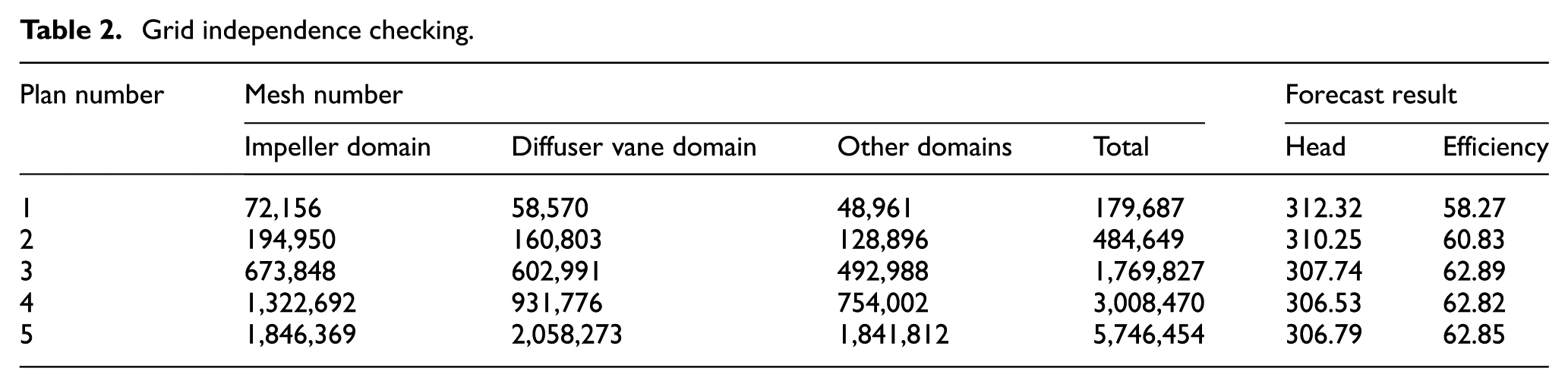
The structured grids, which have the advantages of small truncation error and better convergence, for computational domains are generated using the grid generation tool ICEM14.5. Furthermore, the density of the wall mesh is increased to obtain enough nodes of the wall. The maximum nondimensional wall distance y+< 100 is obtained in the complete flow field. The gap between the hub and the impeller, as well as shroud side chambers, is also included in the grids to take the leakage flow effect into account. The grid details in both rotating and stationary domains are partially shown in Figure 2. The mesh is checked by the grid independence as shown in Table 2. After comparing the accuracy computer calculation time, we chose the third mesh generation method in this present simulation, which has total of 1,769,827 meshes.

Figure 2.

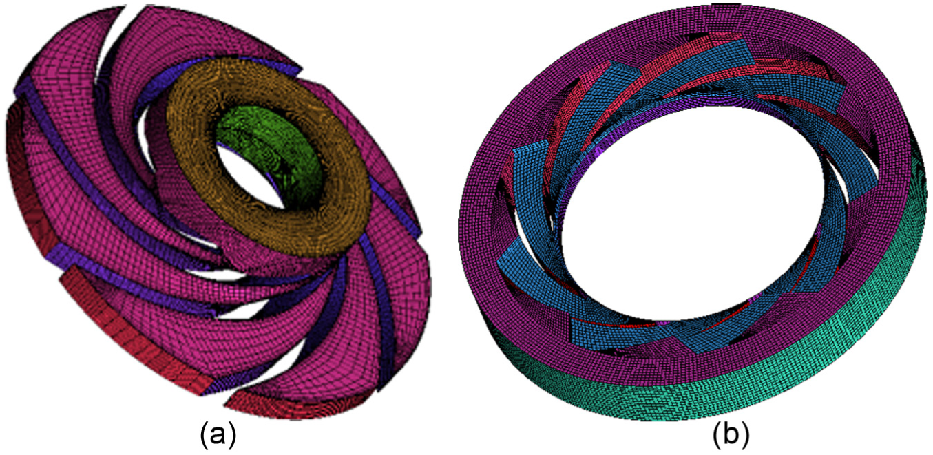
Partial mesh overview of the flow passage: (a) impeller mesh and (b) diffuser vane mesh.

Table 2.

Grid independence checking.

Plan number	Mesh number				Forecast result
Plan number	Impeller domain	Diffuser vane domain	Other domains	Total	Head	Efficiency
1	72,156	58,570	48,961	179,687	312.32	58.27
2	194,950	160,803	128,896	484,649	310.25	60.83
3	673,848	602,991	492,988	1,769,827	307.74	62.89
4	1,322,692	931,776	754,002	3,008,470	306.53	62.82
5	1,846,369	2,058,273	1,841,812	5,746,454	306.79	62.85

Numerical simulation method

The governing equations for the centrifugal pump used to run the numerical simulations are accounted for by making the following assumptions: it has a three-dimensional (3D) incompressible, steady-state flow. Based on these assumptions, these equations can be written as follows:

The continuity equation

\frac{\partial ρ}{\partial t} + \nabla • (ρ \vec{U}) = 0

(1)

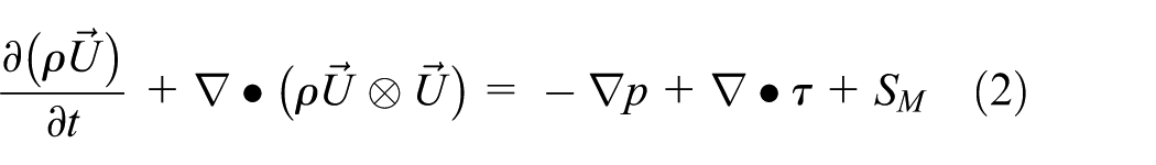
The momentum equation

\frac{\partial (ρ \vec{U})}{\partial t} + \nabla • (ρ \vec{U} \otimes \vec{U}) = - \nabla p + \nabla • τ + S_{M}

(2)

The energy equation

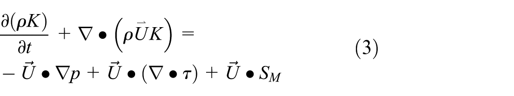
\begin{array}{l} \frac{\partial (ρ K)}{\partial t} + \nabla • (ρ \overset{⇀}{U} K) = \\ - \vec{U} • \nabla p + \vec{U} • (\nabla • τ) + \vec{U} • S_{M} \end{array}

(3)

where ρ is the density, t is the time,τ is the stress tensor, p is the pressure, $\vec{U}$ is the vector of velocity, K is the mechanical energy, and S_M is the momentum source.

The turbulence flow used shear-stress transport (SST) k–ω model, which is based on the k–ω model. The k–ω model has advantages in the low Reynolds number flow calculation because of the treatment of near wall. Also, the model has a function of automatic wall treatment which can choose wall function automatically with different wall conditions. On the base of k–ω model, the SST k–ω model introduces the SST to turbulence model to improve the highly accurate predictions of the onset and the amount of flow separation under adverse pressure gradients. In this article, the calculation domain contains small-scale parts such as the gap of the front cover and the gap of the back cover, and the flow in these parts may change from laminar flow to turbulence flow for the increased velocity and inertial force. Also, the maximum nondimensional wall distance y+ is <100 in the whole calculation domain, which is suitable for SST k–ω model. In addition, SST k–ω model could enclose the Navier–Stokes (N-S) equation if it is assumed that the Newtonian fluid and the thermophysical properties are constant with the temperature. Considering these reasons, the SST k–ω model is accurate and effective in the calculation

\begin{array}{l} \frac{\partial (ρ k)}{\partial t} + \frac{\partial}{\partial x_{j}} (ρ U_{j} k) = \frac{\partial}{\partial x_{j}} [(μ + \frac{μ_{t}}{σ_{k}}) \frac{\partial k}{\partial x_{j}}] \\ + P_{k} - β^{'} ρ k ω + P_{k b} \end{array}

(4)

\begin{array}{l} \frac{\partial (ρ ω)}{\partial t} + \frac{\partial}{\partial x_{j}} (ρ U_{j} ω) = \frac{\partial}{\partial x_{j}} [(μ + \frac{μ_{t}}{σ_{ω}}) \frac{\partial ω}{\partial x_{j}}] \\ + α \frac{ω}{k} P_{k} - β ρ ω^{2} + P_{ω b} \end{array}

(5)

P_{k} = μ_{t} (\frac{\partial U_{i}}{\partial x_{j}} + \frac{\partial U_{i}}{\partial x_{j}}) \frac{\partial U_{i}}{\partial x_{j}}

(6)

μ_{t} = \frac{α_{1} k ρ}{max (α ω, S F_{2})}

(7)

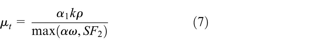
where P_k is the shear production of turbulence; α, α₁, β, β′, σ_k, and σ_ω are the turbulence model constants; k and ω are the turbulence kinetic energy and specific dissipation rate in the k–ω model, respectively; P_kb and P_ωb are the buoyancy production terms; F₂ is the blending function; S is an invariant measure of the strain rate; U is the velocity magnitude; $μ$ is the molecular viscosity; and $μ_{t}$ is the turbulent viscosity.

The steady and transient flow fields of the domain are solved using the CFD code ANSYS CFX14.5. The total pressure is specified to be normal to the boundary at the inlet. At the outlet, the mass flow rate is specified. The roughness of all solid walls is set as no slip is set at 25 µm. The grids of different domains are connected using the general grid interface method. Specifically, the “transient frozen rotor” is set as the interface between the impeller and the volute. First, at the inlet section with 5D₂ length upstream, the impeller is set in a stationary zone with the other sections except for the impeller part which is set as a rotating zone. In the steady simulation, the timescale control uses physical timescale with the value of 0.015923 s corresponding to 5/ω. Then, in the transient simulation, the total time is 0.05 s, and the value of time step Δt chosen for the simulation is 8.33°×°10⁻⁵ s, corresponding to a 3° change in the impeller circumferential position at the nominal rotating speed. The second-order backward Euler scheme is chosen for time discretization. Finally, the convergence criterion is the maximum residual, which is <1 × 10⁻⁵.

Numerical method validations

Test bench

Experimental data have been collected for the high-speed pump that was designed under the initial plan, which has seven impeller blades and nine diffuser vane blades in the laboratory in Shandong Xinyuan Group according to Chinese National Precision grade 2 regulations. Its standard is reported in Table 3.

Table 3.

Test precision standard of grade 2 in China.

Contents	Q	H	P	η
Uncertainty	≤±2.0%	≤±1.5%	≤±1.5%	≤±2.8%

The test rig shown in Figure 3 is tested to pump water out of the experimental pool and eventually flow back through the outlet pipe to the pool. The flow rates are measured by the LWGY-200A turbine flow meter with the measurement error within 0.5%. The pressure is measured by the WT200 intelligent pressure sensor with the precision of 0.1%.

Figure 3.

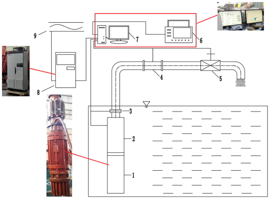
Schematic diagram of test bench.

Results comparison

In order to verify the accuracy of the numerical calculation, a comparison of head and efficiency curves of the pump between the experimental and numerical results is shown in Figure 4. As can be seen from Figure 4, the values of curve and efficiency obtained by the experimental calculation are smaller than those of numerical calculation but according to the same trend. The reason for the errors between the experimental and the numerical values may be due to the following parameters: the 3D model built in the software, the simulation method used in ANSYS, the grid number of the model, and the complex backflow. Taking these parameters into account, the shift is mainly due to the 3D model: the model built progress has ignored the leakage in the mechanical seal. Nevertheless, the obtained numerical results can be considered as acceptable compared to the experimental ones. Despite these assumptions, the numerical method used in this article can explain the nature of the pumping action and help obtain the mechanism of pump’s performance.

Figure 4.

Hydraulic performance comparison of simulated and measured results.

Numerical results

Steady flow field

Figure 5 shows the influence of diffuser vane blade number. In Figure 5, A+B means a combination of the impeller blade number (Z₁ = A) and the diffuser vane blade number (Z₂ = B). This description method is also used in the following parts of this article.

Figure 5.

The effect on pump performance of diffuser vane blade number: (a) Z₁ = 5, (b) Z₁ = 6, and (c) Z₁ = 7.

From the head perspective, 5+8, 6+9, and 7+10 have the highest values in the head curve at all flow rate points, respectively, whereas 5+10, 6+8, and 7+9 have the lowest values in the whole head curves.

From the efficiency perspective, at the design point, the eight diffuser vane blades have the maximum efficiency, and the minimum value point appears in the 10 diffuser vane blades, regardless of the number of impeller blades. It means that the lesser the number of diffuser vane blades, the bigger the flow channel which can pass more water in the same amount of time.

One possible reason for this could be that the more the number of diffuser vane blades, the greater the shock loss. Another reason may be that the narrower flow channel could bring more possibility of blockage. Furthermore, a fluctuation will appear when the impeller passes every diffuser vane blade inlet because of the interference between the static component and the rotating one.

As shown in Table 4, at the design point, when the other parameters remain constant, the maximum efficiency can increase by 3.77%, which appears at the case of seven impeller blades. When Z₁ is 5, the value of head rise is the maximum among the three cases with 2.47%. The reasons for the above phenomenon may be explained as follows: the performance of the pump is affected not only by the coupling between the impeller and diffuser or volume but also by the channel diffusivity of diffuser vane.

Table 4.

Maximum difference of pump performance parameters under different impeller blade numbers.

Z ₁	$\| η_{\max} - η_{\min} \| (%)$	$\| H_{\max} - H_{\min} \| / H_{d} (%)$
5	2.77	2.47
6	3.02	0.71
7	3.77	1.39

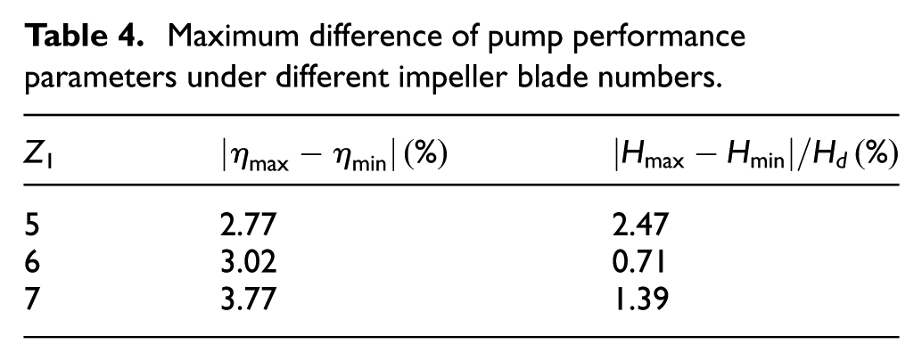
Figure 6 and Table 5 show the influence under different impeller blade numbers. Changing the diffuser vane blade number may have a significant effect on the performance of the pump, when the other parameters are kept constant. Corresponding to the effect exerted by different number of diffuser vane blades, the difference under different impeller blade numbers is more significant. The maximum efficiency difference is 6.45%, and the head difference is 4.49%.

Figure 6.

The effect on pump performance of impeller blade number: (a) Z₂ = 8, (b) Z₂ = 9, and (c) Z₂ = 10.

Table 5.

Maximum difference of pump performance parameters under different diffuser vane blade numbers.

Z ₂	$\| η_{\max} - η_{\min} \| (%)$	$\| H_{\max} - H_{\min} \| / H_{d} (%)$
8	1.56	1.33
9	2.14	3.12
10	6.45	4.49

From the efficiency aspect, in the all three cases with different diffuser vane blade numbers, the case of five impeller blades has the peak efficiency value at the design point. This may be caused by the blade exclusion and surface fiction. But from Figure 5, we found that the efficiency discipline is not strict with the reduced number of impeller blades. For example, under the nine diffuser vane blades, the efficiency of seven impeller blades at the design point is higher than that of six impeller blades. The phenomenon may be attributed to the resonance because of the non-coprime relationship between the impeller blade and diffuser vane blade numbers. In addition, it could also be illustrated that the efficiency of 6+8 is smaller than the case of 7+8.

In Table 6, we see the value and corresponding proportion of hydraulic loss in the whole flow domain. The total loss becomes greater with the increase in diffuser vane number Z₂ when the impeller blade number Z₁ remains constant. The proportion of total hydraulic loss of impeller decreases with the increase in Z₂. The more the diffuser vane blades, the more the hydraulic loss that is caused by impact of the inlet diffuser vane. It could also be noted that there is no strict law in the relationship between impeller blade number Z₁ and related parameters. It is not only the total loss but also the proportion of the impeller hydraulic loss that reaches the maximum value while Z₁ = 6 remains constant. This may lead to the interference following the non-coprime between Z₁ and Z_2.

Table 6.

Hydraulic loss in flow channel.

Impeller blade number, Z₁	Diffuser vane blade number, Z₂	Total hydraulic loss, H_t (mH₂O)	Impeller hydraulic loss, H₁ (mH₂O)		Diffuser vane hydraulic loss, H₂ (mH₂O)		Volute hydraulic loss, H₃ (mH₂O)
Impeller blade number, Z₁	Diffuser vane blade number, Z₂	Value (mH₂O)	Value (mH₂O)	Percentage	Value (mH₂O)	Percentage	Value (mH₂O)	Percentage
5	8	161.69	83.36	51.55	72.41	44.78	5.92	3.66
	9	164.77	82.59	50.12	75.87	46.04	6.31	3.83
	10	180.68	86.3	47.76	88.81	49.15	5.57	3.09
6	8	179.56	103	57.36	70.8	39.42	5.77	3.21
	9	195.30	109.1	55.86	82.16	42.07	4.13	2.07
	10	208.34	108.26	51.96	94.97	45.58	5.11	2.45
7	8	178.19	85.78	48.14	86.6	48.59	5.81	3.26
	9	187.51	87.91	46.88	92.48	49.32	4.38	1.81
	10	190.55	86.11	45.13	97.77	51.31	3.73	3.55

Unsteady flow field

The definition of the flow unsteadiness is based on the pressure fluctuation. For the transient simulations obtained by the unsteady Reynolds-averaged Navier–Stokes (URANS) equations, the pressure fluctuation on the components is only the phase-averaged values. However, the value could respond only to the periodic changing at each grid node in the whole computational domain without instantaneous fluctuating pressure.

Therefore, the periodic unsteady pressure p at a grid node can be decomposed into two parts: one is time-averaged pressure $\bar{p}$ and the other is periodic pressure $\tilde{p}$ which represents the part of the pressure changing periodically with the blade passing frequency. In this article, the two pressures are defined as follows

\bar{p} (node) = \frac{1}{N} \sum_{j = 0}^{N - 1} p (node, t_{0} + j Δ t)

(8)

\tilde{p} (node, t) = p (node, t) - \bar{p} (node)

(9)

\bar{p} (node) = \frac{1}{N} \sum_{j = 0}^{N - 1} p (node, t_{0} + j Δ t)

(10)

To obtain the magnitude and position of the 3D pressure, a root mean square (RMS) number $C_{p_{RMS}}$ is defined as pressure pulsation coefficient. In this article

C_{p_{RMS}} = \frac{\sqrt{\frac{1}{N} {\sum_{j = 0}^{N - 1} \tilde{p} (node, t_{0} + j Δ t)}^{2}}}{\frac{1}{2} ρ u_{2}^{2}}

(11)

where µ₂ is the velocity of the impeller tip, ρ is the density of water, N is the sample number during one revolution period, and t₀ is the starting time of one period of the transient simulation. $C_{p_{RMS}}$ is calculated using the standard deviation. It measures the length of unsteady pressure in a period, which is based on the dimensionless of the dynamic pressure at the impeller exit, regardless of the particular instantaneous position of the impeller rotation.

Figure 7 shows the distribution of pressure fluctuation intensity on the mid span of impeller and diffuser vane at the design condition. From Figure 7, we see that the distributions present the same regular pattern. From a macro perspective, the pressure fluctuation increases with the growth of the radius. It means that with the high rotation of the impeller, the movement becomes increasingly intense. Furthermore, in most cases, the fluctuations reach the peak value at the inlet of the diffuser vane flow channel which is expressed by the violent impact that occurs when the fluid enters the diffuser vane. Due to the flow pattern, the strength of the flow may be affected by the velocity, the shape of inlet angle of diffuser vane, and so on. The evident differences among the nine cases show the influence in various cases.

Figure 7.

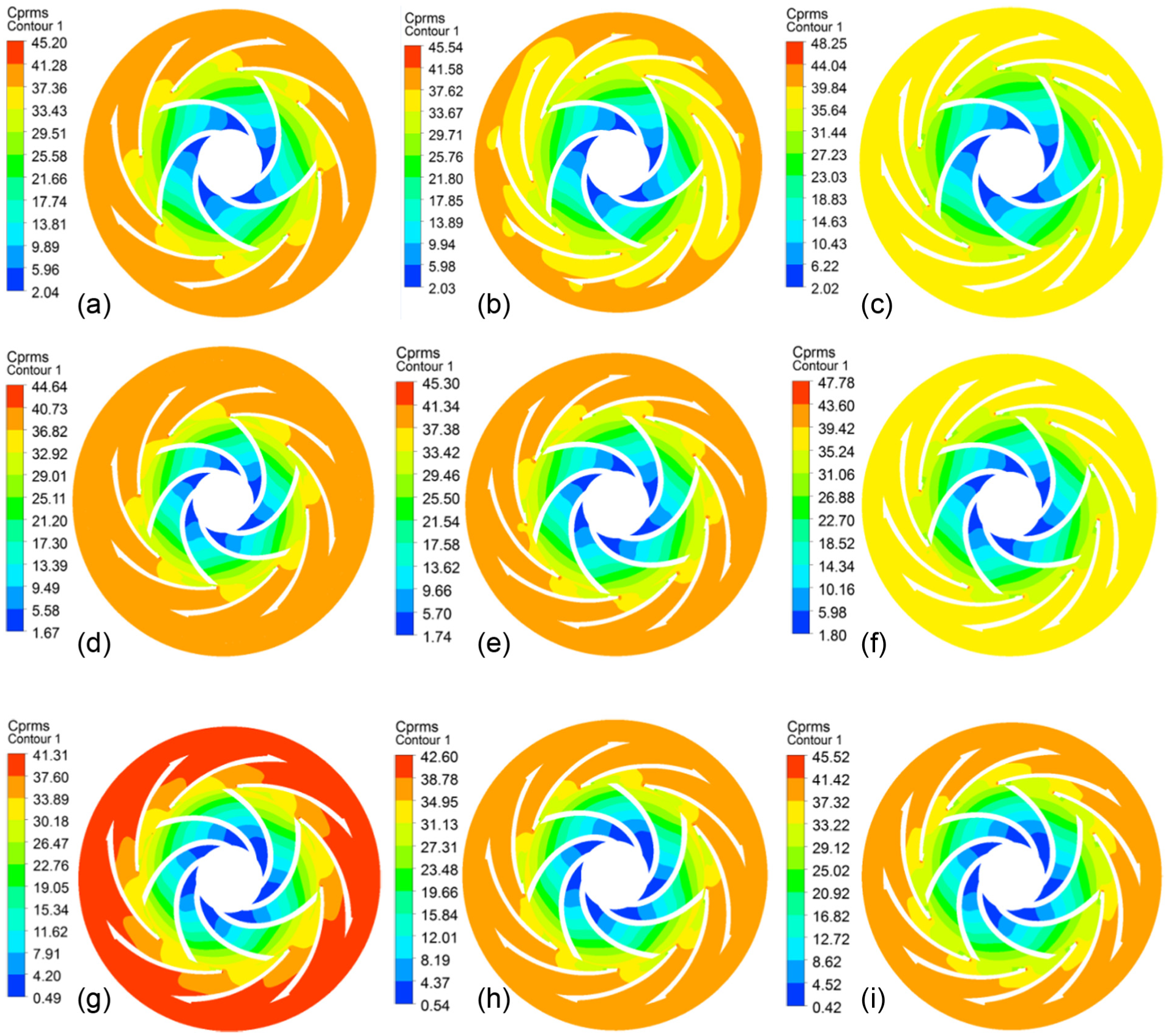
Pressure fluctuation intensity at impeller mid span = 0: (a) 5+8, (b) 5+9, (c) 5+10, (d) 6+8, (e) 6+9, (f) 6+10, (g) 7+8, (h) 7+9, and (i) 7+10.

Furthermore, we see that with the increase in the number of diffuser vane blades, the maximum intensity becomes larger. Similarly, the minimum decreases with the decrease in the number of impeller blades. From the individual case, the peak value of $C_{p_{RMS}}$ emerges in the case of 7+8 attributes to no intense fluctuation in the inlet angle of diffuser vane.

The hydrodynamic force acting on the surface of the structure is the resultant of the fluid pressure and the fluid viscous force acting on the rotating and stationary surfaces. This article assumes that the resultant force in the radial plane is equivalent to the axis of the impeller shaft ignoring the effect of impeller eccentricity. The radial force of impeller is the integration of these dispersion forces in the surface, which is a function affected by the impeller rotation position and time.²⁵

The form is

F_{p} = - \int_{A} p • e • dA

(12)

F_{v} = - μ \int_{A} (\frac{d μ}{d n_{n}}) • e • dA

(13)

F_{r} = F_{p} + F_{v}

(14)

where F_r is the radial force, F_p is the radial force caused by the fluid pressure, and F_v is the radial force caused by the fluid viscosity.

The interaction between the rotor and stator is the main source of the flow unsteadiness, as can be inferred from the periodicity of the radial force. Figure 8 shows the radial force fluctuation along the X and Y axial directions under the nine different matching cases between the blade number of impeller and diffuser vane under the initial five cycles when the pump worked at the design point.

Figure 8.

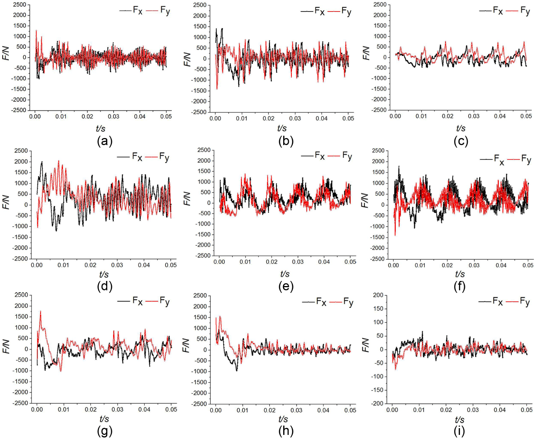
Radial force fluctuation: (a) 5+8, (b) 5+9, (c) 5+10, (d) 6+8, (e) 6+9, (f) 6+10, (g) 7+8, (h) 7+9, and (i) 7+10.

This can be seen easily from Figure 8 that the radial fluctuation presents periodicity approximately except the unsteady first cycle. From the aspect of fluctuation value, in addition, when we only change the number of impeller blade or diffuser vane blade, the difference in fluctuation is huge. The value fluctuates between negative 500 N and positive 500 N when the number of impeller blade is 7, which is the minimum value among the different impeller blade number series. The maximum fluctuation appears when the number of impeller blade is 6, with the value in a range between negative 1500 N and positive 1500 N.

The difference among the fluctuation gradients in the nine cases stands for the operational stability. Furthermore, it can also be considered that the smaller the gradient means the better the stability. The difference may be caused by the following reasons: the return flow and impulse loss occur at the exit of the impeller runner and the inlet of the guide vanes; the magnitude of the return strength; and the impact loss constantly changing with the high-speed rotation of the impeller, so that the radial force does not agree with the amplitude value.

From the aspect of fluctuation distribution, most situations of the different blades matching present a periodic characteristic after the first unsteady cycle. However, the force fluctuation in some cases such as 7+10 is not in accordance with an evident periodical phenomenon. This may be caused by the irregular interference following the resonance between the impeller and diffuser vane.

Referring to the above occurrence, it may be caused by the following reasons:

An eddy appears in the impeller channel or the gap between the outlet of impeller and inlet of diffuser vane. The eddy is exerting influence on the flow field with the high-speed rotation;

There is turbulence in a certain impeller channel that leads to a blockage in the channel.

Conclusion

Different matching patterns of blade numbers between impeller and diffuser vane in a high-speed rescue pump, which is a new product in this field, are studied in this article. In total, nine cases combined with different impeller blade numbers (Z₁ = 5, 6, 7) and diffuser vane blade numbers (Z₂ = 8, 9, 10) are analyzed by numerical simulation. The results from the comparisons show that

At the design point, in most cases, the efficiency increases with the reduction in the impeller blade number when the other parameters remain constant. This law is also applicable to the decreased blade number of the diffuser vane. However, some specific matching cases do not obey the law possibly due to the interference between the impeller and diffuser.

At the design point, when the impeller blade number changes and the other geometry parameters of the high-speed rescue pump remain constant, the head increases from the minimum to maximum at the percentage of 2.47%, 0.71%, and 1.39%, respectively. As for the efficiency, it increases with the percentage of 2.77%, 3.02%, and 3.77%, respectively. When the diffuser blade number changes and the other parameters remain constant, the largest variation ranges of head are 2.47%, 0.71%, and 1.39%, and the maximum variations of efficiency are 2.77%, 3.02%, and 3.77%, respectively.

The pressure fluctuation intensity in the nine cases reveals the inner flow status in the flow channel. The largest fluctuation occurs near the inlet of diffuser vane channel due to the rotor–stator interaction. Furthermore, the 7+8 case has the minimum fluctuation attributed to its good matching.

The radial force almost changes at a range between negative 1500 N and positive 1500 N. The relative small radial forces appear under the seven impeller blade series compared to other cases.

Therefore, 7+8 case is the best choice considering both steady and unsteady results.

Footnotes

Appendix 1

Academic Editor: Ming-Jyh Chern

Declaration of conflicting interests

The author(s) declared no potential conflicts of interest with respect to the research, authorship, and/or publication of this article.

Funding

The author(s) disclosed receipt of the following financial support for the research, authorship, and/or publication of this article: This work was partly supported by the grants of National Natural Science Foundation of China (no. 11602097) and Jiangsu Natural Science Foundation (no. 6156304).

References

Dong

SN.

Current situation and prospect of coal mine geological guarantee technologies to improve safety and efficiency. Coal Sci Technol 2007; 35: 1–5.

Peng

SP.

Present study and development trend of the deepen coal resource distribution and mining geologic evaluation. Coal 2008; 17: 1–11.

Jin

Liu

Wang

Development and prospect of coal deposit hydrogeology. Coal Geol Explor 2009; 37: 28–31.

Progress, problems and prospects of prevention and control technology of mine water and reutilization in China. J China Coal Soc 2014; 39: 795–805.

Feng

Benra

Dohmen

HJ.

Investigation of periodically unsteady flow in a radial pump by CFD simulations and LDV measurements. J Turbomach 2011; 133: 1–4.

Iannetti

Stickland

Dempster

. A CFD study on design parameters acting in cavitation of positive displacement pump. In: Proceedings of the 12th European fluid machinery congress, Edinburgh, 6–7 October 2014, pp.143–157. Woodhead Publishing Limited.

Junaidi

MAR

Kumari

NBVL

Samad

MA.

CFD simulation to enhance the efficiency of centrifugal pump by application of inner guide vanes. Mater Today Proc 2015; 2: 2073–2082.

Shah

Jain

Patel

CFD for centrifugal pumps: a review of the state-of-the-art. Procedia Engineer 2013; 51: 715–720.

Barrios

Scott

Sheth

KK.

ESP technology maturation: subsea boosting system with high GOR and viscous fluid. In: Proceedings of the SPE annual technical conference and exhibition (vol. 2), San Antonio, TX, 8–10 October 2012, pp.1580–1601. Society of Petroleum Engineers (SPE).

10.

Maitelli

Bezerra

Mata

WD.

Simulation of flow in a centrifugal pump of ESP systems using computational fluid dynamics. Braz J Petrol Gas 2010; 4: 1–9.

11.

Sirino

Stel

Morales

REM

. Numerical study of the influence of viscosity on the performance of an electrical submersible pump. In: Proceedings of ASME 2013 fluids engineering summer meeting (vol. 1B), Incline Village, NV, 7–11 July 2013. New York: ASME.

12.

Stel

Sirino

Ponce

FJ.

Numerical investigation of the flow in a multistage electric submersible pump. J Petrol Sci Eng 2015; 136: 41–54.

13.

Stel

Sirino

Prohmann

. CFD investigation of the effect of viscosity on a three-stage electric submersible pump. In: Proceedings of American Society of Mechanical Engineers, fluids engineering division (publication) FEDSM (vol. 1B), Chicago, 3–7 August 2014. American Society of Mechanical Engineers (ASME).

14.

Zhu

Hattan

Xia

ZY.

CFD simulation and experimental study of oil viscosity effect on multi-stage electrical submersible pump (ESP) performance. J Petrol Sci Eng 2016; 146: 735–745.

15.

Pinedaa

Biazussib

Lópezb

Phase distribution analysis in an Electrical Submersible Pump (ESP) inlet handling water–air two-phase flow using computational fluid dynamics (CFD). J Petrol Sci Eng 2016; 139: 49–61.

16.

Verde

WM.

Experimental study of BCS pumps operating with biphasic gas-liquid flow. Campinas, Brazil: State University of Campinas, 2011.

17.

Gamboa

Mauricio

Experimental study of two-phase performance of an electric-submersible-pump stage. SPE Prod Oper 2012; 27: 414–421.

18.

Zhou

Sachdeva

Simple model of electric submersible pump in gassy well. J Petrol Sci Eng 2010; 70: 204–213.

19.

Ziegler

Gallus

Niehuis

. Study on impeller-diffuser interaction: part I—influence on the performance. In: Proceedings of the ASME Turbo Expo (vol. 5), Amsterdam, 3–6 June 2002, pp.545–556. New York: ASME.

20.

Shum

YKP

Tan

Cumpsty

. Impeller-diffuser interaction in a centrifugal compressor. In: Proceedings of the ASME Turbo Expo (vol. 1), Reno, NV, 6–9 June 2000. New York: ASME.

21.

Casey

Rusch

The matching of a vaned diffuser with a radial compressor impeller and its effect on the stage performance. J Turbomach 2014; 136: 121004.

22.

Zhang

Numerical analysis of fluid structure interaction and comments to rotor stator interaction in AP1000 reactor coolant pump. Dalian, China: Dalian University of Technology, 2012.

23.

Wang

Yuan

Pei

Hydraulic performance study on matching of impeller and diffuser of residual heat removal pump. J Huazhong Univ Sci 2015; 43: 39–43.

24.

Yang

Wang

Zhang

ZH.

Computational fluid dynamics analysis of effects of number of pump blades on water-jet propeller performance. J Mech Eng 2009; 45: 222–228.

25.

ANSYS, Inc. ANSYS user manual 12.0. Canonsburg, PA: ANSYS, Inc., 2009.

Effect of blade number matching of impeller and diffuser in high-speed rescue pump

Abstract

Keywords

Introduction

Physical model

Numerical approach

Three-dimensional model built

Mesh dividing

Numerical simulation method

Numerical method validations

Test bench

Results comparison

Numerical results

Steady flow field

Unsteady flow field

Conclusion

Footnotes

Appendix 1

Declaration of conflicting interests

Funding

References