
Abstract
This article presents a calibration model for the whole grinding system to enhance its accuracy, because of the problem of low accuracy of the robotic belt grinding system which is due to the low absolute positioning accuracy of the robot as well as the deformations of the turbine blades and grinding tool under the grinding force. First, the transition matrix of system working accuracy was established and the corresponding evaluation criterion was put forward for the systemic features. Then the deformation of the turbine blades and grinding tool were analyzed and modeled, respectively, and the model of the absolute positioning accuracy of the robot was established based on the geometrical error as well as the compliance error. Finally, based on the models above, a method of error compensation was presented and the flowchart was given. The experiments show that the absolute positioning accuracy of the robot (the average value reduces from 1.186 to 0.154 mm) and the accuracy of the whole grinding system (the average grinding force is 20.4 N which is very close to the predetermined 20 N) have been effectively improved, which prove that the method can help to expand the application scope of the robotic system.
Introduction
Complex thin-walled components such as turbine blades and aero-engine cases are becoming increasingly widely used in aerospace industries. 1 This kind of components is characterized by multi-variety and small batch. The cost of traditional Computer Numeric Control (CNC) machining is high and difficult to expand into new objects, which makes it not suitable for these components. 2 For the characteristics of such components, the industrial robot gets an ever-increasing concern and is becoming more and more widely used nowadays because of its low cost, flexibility, and versatility.3–6 The robotic belt grinding system for turbine blades is a typical case.
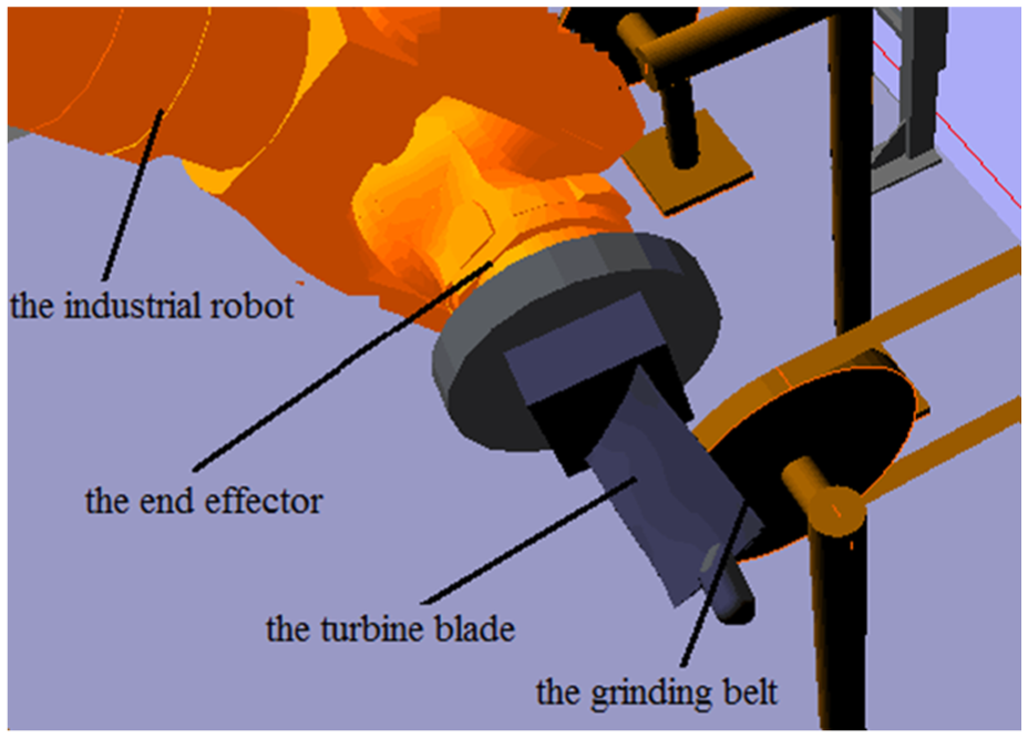
The robotic belt grinding system for turbine blades mainly consists of three parts, namely, the industrial robot, turbine blades, and the grinding tool, which includes the grinding belt and the grinding wheel. In this system, the industrial robot belongs to flexible manufacturing equipments and its accuracy indexes include the repeated positioning accuracy and absolute positioning accuracy. The grinding of turbine blades is mostly based on the off-line programming, and the grinding paths always need to be adjusted accordingly which places greater demands on the absolute positioning accuracy.7,8 Generally, the repeated positioning accuracy of industrial robots is high, while the absolute positioning accuracy is low which cannot meet the grinding requirement of turbine blades. 9 The other two parts, turbine blades and the grinding tool, are both flexible bodies. They suffer from the elastic deformation during the grinding process due to their low stiffness, which makes the actual grinding position deviate from the predetermined one. Based on the analysis above, the flexibility of the three parts will lead to a decline of the system accuracy and make it difficult to meet the high-accuracy requirement of blades grinding. Therefore, it is necessary and meaningful to perform further studies on the working accuracy of robotic belt grinding system.
Most current studies focus on the robot alone and enhance the robotic positioning accuracy by modifying the kinematic parameters in the selected calibration space.10–12 Known from the analyses above, the working accuracy for robotic belt grinding system is affected by the combination of the industrial robot, turbine blades, and the grinding tool. Therefore, the positioning accuracy of the robot alone cannot reflect the performance of the entire system and the error compensation of the robot can neither necessarily enhance the working accuracy of the entire system.
To solve the problem above, this article presents a calibration model of the whole system from the systemic point of view. A transition matrix of the system working accuracy and the corresponding evaluation criterion are put forward first. The deformations of turbine blades and the grinding tool as well as the absolute positioning accuracy of the robot are also modeled, respectively. Based on the models above, the method of the error compensation for the entire system is presented. Finally, the results of the grinding experiments are discussed and the summary of major contributions from present work is concluded.
Modeling of the working accuracy
In this section, a transition matrix of system working accuracy is established first and the evaluation criterion is put forward for the systemic features. As analyzed above, the working accuracy of the whole system is affected by the industrial robot, turbine blades, and the grinding tool together, therefore the three parts will also be modeled in this section.
The working accuracy of the system
The working accuracy, different from the accuracy indexes of the robot, is used to describe the processing performance of the entire system, namely, the ability to complete the grinding tasks. Grinding is a process of the material removal by the contact between the blades and grinding belt. The contact location is called the “working point” which has a direct impact on the accuracy of the grinding system.
The transition matrix of the working accuracy
In order to describe the system shown in Figure 1 more conveniently, the Cartesian coordinate system is established here:
Base coordinate system. The coordinate system for the robot base which is fixed on the ground;
End coordinate system. The coordinate system for the end-effector of the robot;
Belt coordinate system. The coordinate system for the grinding tool. In this article, the grinding tool is fixed on the ground;
Blade coordinate system. The coordinate system for the turbine blades; the blade is held by the end-effector of the robot, therefore the blade coordinate system changes as the robot moves;
Work coordinate system. The coordinate system for the contact location between the blades and the grinding belt. It changes with the “working point.”
Schematic diagram of the grinding system.
For different “working points,” the relationship of the coordinate systems above is as follows

where
Making a transformation to equation (1), the following equation can be obtained

where
In equation (2),
The evaluation criterion of the working accuracy
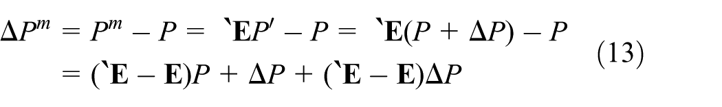
In the robotic grinding system, the actual working matrix is

The “working error” is used to characterize the deviation between the actual “working point” and the ideal one of the grinding system. The smaller the

where
In the actual grinding process, the real-time detection of the “working points” is difficult due to the continuity of the process and therefore the matrix of

where
The deformation models of the blades and grinding tool
The turbine blades belong to the complex thin-walled components. The deformation is difficult to be predicted by specific equations. Here in this work, commercial FEA package ANSYS has been used along with its design language (APDL) environment and automatic mesh generation routine to predict static deflections of the blade.
The material of the turbine blades is titanium alloy whose properties are easy to know. The distribution of the grinding force on the blade is complex. In this article, the grinding tool and the blade are both with a definite elasticity, and the contact between them is assumed to obey the Hertzian contact theory.16,17 Therefore, the distribution of the grinding force on the blade can be obtained according to the Hertzian contact theory which is not discussed here for the limitation of the length.
As these parameters are known, using the commercial FEA package ANSYS, the deformation of the blade under certain grinding force can be obtained, which is shown in Figure 2. In the simulation, the grinding force of 20 N was adopted and the biggest deflection happened when the grinding force was applied on the very edge of the blade as shown in Figure 2(b). It can reach as big as 0.08 mm which is almost half of the error of the absolute positioning accuracy of the robot after the compensation as shown in Table 2 (see the “Experiments and discussion” section). Therefore, it indicates that the deflection of the blade has a great effect on the overall accuracy of the grinding system and cannot be neglected.

Schematic diagram of the deformation of the blade based on the finite element analysis method: (a) The model of the blade and (b) the deformation of the blade.
As for the characteristics of the grinding tool, the flexible body usually refers to the grinding wheel. The contact wheel is usually composed of a stiff core and an elastic cover which will get deformed under the grinding force. If the deformation is small enough, it can be regarded as a wholly elastic deformation. 18 The calculation of the elastic deformation can be transformed into a Signorini problem, a contact problem between an elastic body and a rigid body, which is illustrated by Figure 3.18,19 Here, the classical theoretical model of strain–stress as well as the energy minimization principle which defines the way how a constrained object deforms with the effect of external forces is applied to solve the problem.

Schematic diagram of the deformation of the grinding tool. 18
In Figure 3,

where
The model of the absolute positioning accuracy of the robot
Based on the analyses of the deformation of the blades and grinding tool, the matrixes of
There are many factors that can affect the absolute positioning accuracy of the robot, such as temperature error, geometrical error, as well as the compliance error caused by the weight of the robot and external loads. 21 Therefore, it is hard to establish a model that contains all the factors. Studies have shown that the maximum error of the robot comes from the geometrical error, while the compliance error cannot be ignored either. 22 There is a coupling between them and geometrical error is always accompanied by the compliance error which changes with the position and orientation of the robot all the time, leading to a difficulty in distinguishing the two errors. Many studies just simplify this situation and consider the two kinds of error as one which makes the result imprecise.21,23
To solve these problems, an error model on the basis of relative positions is presented in this section which uncouples the geometrical error from the compliance error. And then a model of the compliance error is established. The two models together determine the overall error of the robot.
The error model on the basis of relative positions
The error model of the robot is based on the kinematics, using Modified D-H (MD-H) method which is based on the D-H method and introduces a rotational parameter around the Y axis to avoid the singular value when the adjacent joints are parallel. 21 Figure 4 is the coordinate system for the joints of the KR 210 R2700 robot from the company of KUKA.

The coordinate system for joints of KR 210 R2700 based on the MD-H model.
According to the MD-H model, the transformation equation between the successive reference systems can be expressed as follows 24

where
For n-joints robot, the transformation equation from the end coordinate system to the base coordinate system can be written as follows

Equation (8) is the transformation equation in the ideal case. While the manufacturing and assembly errors of the robot can lead to the geometrical error, the real transformation equation from the end to the base coordinate system can be obtained as follows
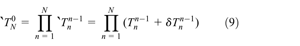
where
When the geometrical errors are small,
21

where
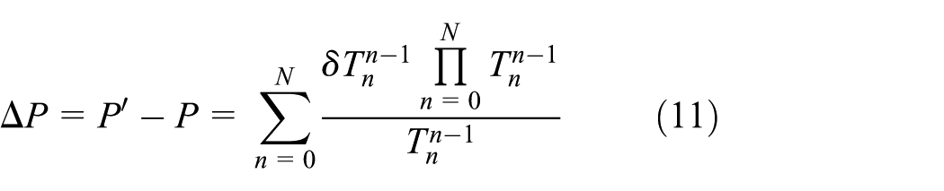
Based on equations (7)–(10), omitting the high-level minim, the error between the actual position
In the process of measurement, the laser tracker is mostly used to construct the base coordinate system of the robot. 25 In previous studies, it is assumed that the base coordinate system constructed by the laser tracker is the same with the real one. However, in practice, it is impossible to make the two coordinate systems coincident with each other perfectly.7,21 In order to reduce the transformation error, a coordinate transformation matrix between the two coordinate systems is introduced as follows
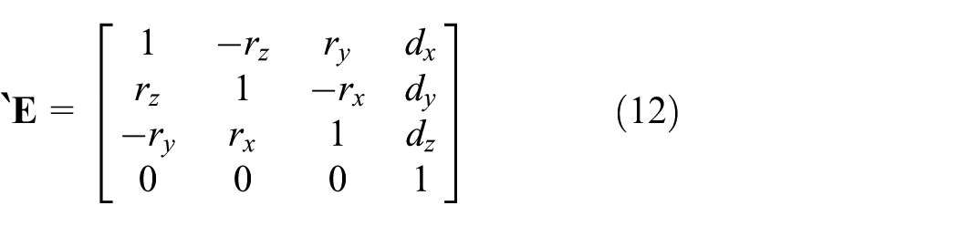
where
Considering the measurement error, the absolute positioning error equation for a single location can be expressed as follows
where

As analyzed before, there is a coupling of compliance error in equation (14) which needs to be eliminated.
The compliance error comes from the deflection of the robotic links and joints caused by the weight of the robot and external loads. 26 In belt fine grinding process, the grinding depth is very small, leading to a small grinding force which is usually under 100 N. 27 Compared with the weight of the robot, the grinding force can be neglected in this part. In addition, the links can be approximated as rigid bodies whose deflection can be ignored too. 28 Therefore, the deflection of joints caused by the weight of the robot is taken into consideration in the compliance error.
The second and the third are the heaviest among all the links of the robot. So the torques on the second and third joints are the biggest as well as the corresponding deflection of them. 22 Therefore, the model of the compliance error can be simplified further by only considering the deflection of the second and third joints caused by the weight of the second and third links.
For the features of the compliance error, the geometrical error model on the basis of relative positions can be established here. At two different locations, the theoretical coordinates of the end-effector are
The relative error of the two locations can be obtained as follows
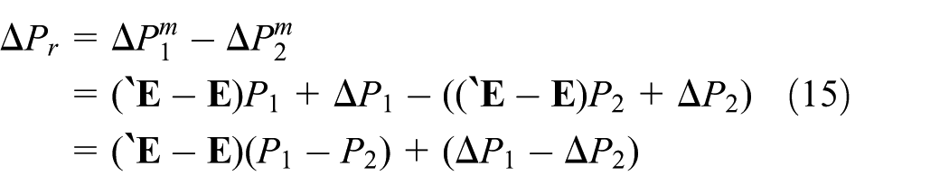
Equation (15) is the error model on the basis of relative positions. In this model, as analyzed above, when the coordinates in the vertical space, namely, the vertical height in the base coordinate system, of the second and third joints for two locations are approximately equal, it can be assumed that the torques on the second and third joints are the same, which means the compliance error caused by the weight of the robot is equal. Then the error model on the basis of relative positions can eliminate the effect of the compliance error on the geometrical error.
The model of the compliance error
According to the analysis above, the deflections of the second and third joints caused by the weight of the second and third links are considered in the model of the compliance error.
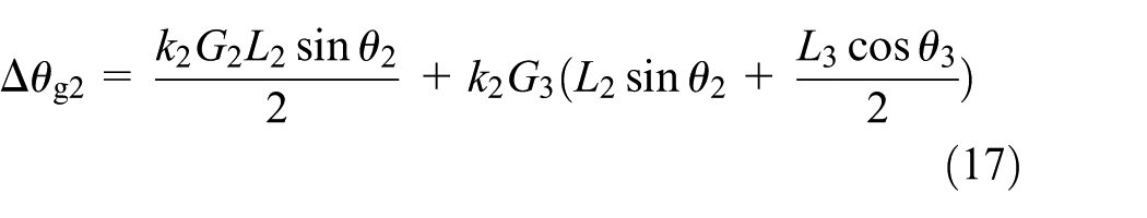
Related studies have shown that the torsion angle of the joint is proportional to the torque on it. 29 Thus in this part, the torsion angle can be expressed as follows

where
As shown in Figure 5, it is assumed that

Schematic diagram of self-gravity compliance error.
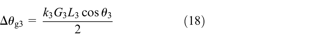
Similarly, the torsion angle of joint 3 can be written as follows
The error compensation method for the grinding system
Based on the analyses above, a method to characterize the working accuracy of the grinding system was presented and three models were established to describe the flexible parts of the system. In this section, an error compensation method for the grinding system is presented as shown in Figure 6:
Step 1. Based on the analysis of the deformation of the blade and the grinding tool, the actual contact point can be obtained.
Step 2. Based on the actual contact point, the coordinate of the end-effector of the robot can be calculated.
Step 3. Make calibration for the robot by following the steps that are detailed below: Collect the coordinates of the end-effector and calculate the errors of the geometrical parameters based on the error model on the basis of relative positions. Implement the load tests to obtain the elasticity coefficients of joints 2 and 3, and then calculate the compliance error based on equations (17) and (18). Change the nominal parameters of the robot based on the results in steps 1 and 2, a new set of parameters can be obtained. Recalculate the absolute positioning accuracy of the robot according to the new set of parameters. Stop when the error value

The flowchart of the error compensation method for the grinding system.
Experiments and discussion
The experiments of the absolute positioning accuracy for the robot
First, the experiments for the calculation of the geometrical parameters errors were conducted. All the experiments were performed on the robot of KR 210 R2700 and the coordinates of the end-effector were measured by the API laser tracker as shown in Figure 7. First, the laser tracker was used to conduct the base coordinate system. Then, different coordinates of the end-effector were put into the controller of the robot and the real coordinates could be obtained by the laser tracker. Finally, according to the error model on the basis of relative positions, the geometrical parameters errors for the robot could be calculated.

The experimental scene of the precision calibration for the robot.
A total of 11 groups of samplings are needed at least according to the requirement of the minimum samplings. 21 In this article, 20 groups of samplings were selected to make the results more precise. The geometrical parameter errors for the robot of KR 210 R2700 are listed in Table 1.
The geometrical parameter errors of KR 210 R2700.

The load tests are implemented to calculate the elasticity coefficients. The posture of the robot is not changed, and then different weights are loaded on joints 2 and 3. The API laser tracker is used to detect the coordinates of joints 2 and 3 before and after the load tests. According to equations (17) and (18), the results are as follows

The elasticity coefficients are taken into the model of the compliance error, and the compliance errors

Schematic diagrams of the compliance errors
As shown in Figure 8, the compliance errors exist all the time and change with the posture of the robot. It can be seen that the biggest error for the torsion angles can reach 0.08° which is almost the same with the geometrical error of the rotational angle for joint 4. Therefore, the compliance errors have a great effect on the positioning accuracy of the robot and cannot be neglected.
Based on the error compensation method in this article and Gong et al., 21 20 groups of samplings were compensated separately and the results can be seen in Figure 9 and are listed in Table 2.

The absolute positioning errors before and after the error compensation by different methods.
The results of the absolute positioning accuracy by different compensation methods.

As we can see from Table 2, after the compensation by the two methods, the absolute positioning accuracy of the robot has been greatly improved. Compared with the method by Gong et al., 21 the maximum and average values in this article is smaller, which means that the method in this article has a better effect.
The experiments of the working accuracy for the system
As we have stated, the grinding force is chosen as the measured parameter of the system accuracy. Here in the experiments of this article, the force controller of ACF 110-10 produced by FerRobotics Company as shown in Figure 10(a) was used to detect the grinding force. In general, ACF is fixed at the end-effector of the robot as shown in Figure 10(b). Through the integration of multiple sensors, the reaction time of ACF can be as short as 4 ms which guarantees that it can make feedback in real-time to the robot and finally achieve precise control of the force through the control software, as shown in Figure 10(c).

The objective picture of ACF 110-10 and its usage on the robot: (a) the objective picture of ACF 110-10, (b) the usage of ACF on the robot, and (c) the control surface of ACF.
The grinding force is set to be 20 N. There are three parts in the experiments and each of them contains 20 “working points.” The results are shown in Figures 11–13.
The grinding forces in the first part of the experiments.
The grinding forces in the second part of the experiments.

The grinding forces in the third part of the experiments.
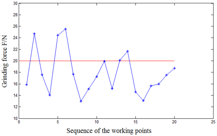
In the first part of the experiments, there is no calibration on the robot, and the grinding tool and the blades are considered to be rigid bodies where no deformation is taken into consideration. Figure 11 is the result of the grinding force under this situation.
As we can see from Figure 11, the grinding force varies in a comparatively large range. The maximum it can reach is at 25.8 N and the minimum at 11.4 N. Compared with the predetermined value of 20 N, the grinding forces under this situation cannot meet the requirement of the blade grinding.
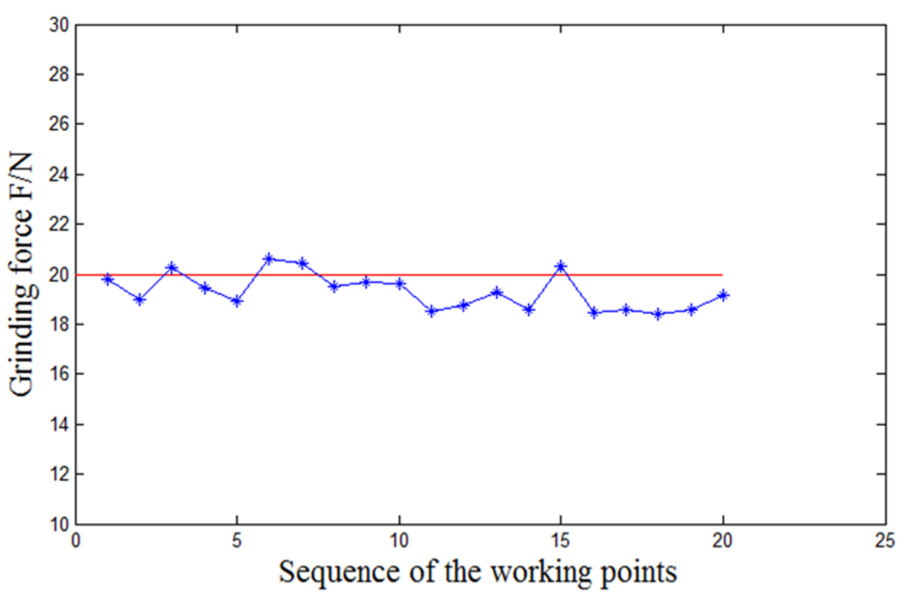
In the second part of the experiments, the robot is calibrated, while the deformation of the grinding tool and the blades is not taken into consideration. Figure 12 is the result of the grinding force under this situation.
In Figure 12, the maximum of the grinding forces is at 20.8 N and the minimum is at 17.9 N. Compared with the result of the first part, the grinding force in this part varies within a much smaller range which is because of the calibration of the robot. However, the grinding force is generally lower than 20 N which can be explained by that the elastic deformation of the grinding tool and the blades lead to a smaller contact between them.
In the third part of the experiments, the method of system calibration in this article is adopted, which means the robot is calibrated and the deformation of the grinding tool and the blades is taken into consideration. Figure 13 is the result of the grinding force under this situation.
As we can see, there is a fluctuation of the grinding force in this part too, which is because the absolute positioning error of the robot cannot be eliminated completely. Compared with the results of the second part, the grinding force in this part varies near the predetermined value of 20 N. The average grinding force is 20.4 N, which is very close to the predetermined value that can meet the requirement of the blade grinding and verify the model of this article.
Conclusion
From the systemic point of view, a model of the working accuracy for robotic belt grinding system for turbine blades is presented and the following tasks have been performed in this article:
The transition matrix of system working accuracy is established and the evaluation criterion is put forward.
The elastic deformations of the blade and the grinding tool are individually modeled to obtain the actual contact point.
As for the feature of the robot, two error models are established: the error model on the basis of relative positions and the model of compliance error. They together characterize the absolute positioning accuracy of the robot.
Based on the error models above, an error compensation method for the system is presented.
The experimental results show that through the calibration method in this article, the absolute positioning accuracy of the robot can be greatly improved, which will help to expand its application into the area of precision finishing such as assembly and measurement. The compensation method in this article can improve the accuracy of the belt grinding system and makes the system meet the requirement of the blade grinding. Therefore, the method can also expand the application scope of the whole grinding system.
Footnotes
Academic Editor: Duc T Pham
Declaration of conflicting interests
The author(s) declared no potential conflicts of interest with respect to the research, authorship, and/or publication of this article.
Funding
The author(s) disclosed receipt of the following financial support for the research, authorship, and/or publication of this article: This study was supported by the Fundamental Research Funds for the Central Universities (Grant No. 3102015JCS05012).