Calibration and error compensation of scanner-based robotic belt grinding system

Abstract

Turbine blade is one of the key components of turbomachinery, and the machining quality of its airfoil surface has an important impact on the operating efficiency, service life, and safety of the turbine. Robotic abrasive belt grinding has become an important means of blade airfoil surface machining. Based on the self-developed robot grinding system, this paper proposes a scanner-based system calibration method to determine the relationships among coordinate systems of measurement, robot base, tool, and workpiece. An accurate and efficent calibration method of workpiece coordinate system based on rapid surface segmentation of point cloud using CAD model is established. An blade error surface is constructed by B-spline interpolation to compensate system errors such as absolute positioning error of robot, calibration error, and blade shape error. The calibration process is illustrated at the end of this paper. The effectiveness of the calibration and error compensation methods proposed in this paper are verified by the simulation results.

Introduction

Blade is one of the key turbomachinery components. Its manufacturing quality directly affects the core turbine performance. The blade works in the harsh environment of high temperature, pressure, and speed. Its design and manufacturing process needs to meet the performance indexes of aerodynamics, heat transfer, and structure. Therefore, the blade is always accompanied by complex structural surface, high processing difficulty, and long manufacturing cycle. In order to meet the ultra-high requirements of turbine blades for performance, safety, reliability, and service life with many varieties and large quantity, the blade manufacturing technology should be continuously improved.

Robotic abrasive belt grinding has become an important means of blade airfoil surface finishing. Taking the steam turbine blade as an example, most of the operations are done in the machining center from a minimum envelope stainless steel blank except for the finishing of airfoil surfaces. Successful belt grinding involves many aspects such as coordinate system calibration, ¹ grinding process modeling, ² trajectory planning,^3–5 grinding force adaptive control, ⁶ error analysis, and compensation.^7,8 In order to achieve the practical application of the belt grinding system, the first step is to establish an efficient, accurate, and practical coordinate system calibration method.

The calibration of abrasive belt grinding system is mainly used to determine the relationships among coordinate systems of robot, measurement, blade workpiece, and belt grinder. The robot and measurement equipment can be pre-calibrated individually before joining the grinding system.^9,10 Robotic belt grinding system is a typical “hand-eye” system. The traditional robot hand-eye calibration is to solve a homogeneous equation AX = XB or AX = YB, where X and Y are the unknown hand-to-camera rigid transformation and the robot-to-world rigid transformation, respectively, and A and B are the movements of the hand and camera, respectively ¹ . Li et al. ¹¹ calibrated the coordinate system relationship between the robot end effector and the scanner with a calibration ball, and also gave the robot joint error in the calibration process. The measurement equipment and belt grinder are generally fixed on the ground due to the grinding dust and the larger volume and mass of belt grinder, and, therefore, the blade is installed at the end of the robot flange. This configuration increases the difficulty of calibrating the relationship between coordinate systems of robot and tool. Xu et al. ¹² took the ruby probe fixed on the robot flange as the main calibration tool, calibrated the ruby probe through the calibration ball fixed on the ground, and then calibrated the coordinate system of the belt grinder with the ruby probe. The calibration of the workpiece coordinate system is obtained by solving the transformation relationship between several blade contour points measured by the ruby probe and the corresponding points in blade CAD model. The above calibration process is clear, but the accuracy of actual blade contour points is poor due to machining errors, and the calibration results of blade workpiece coordinate system may fluctuate. The difficulty of belt grinding system calibration lies in how to complete the whole calibration process accurately, quickly, and make it easy to realize automation.

Due to the pose error brought by blade installation, it is necessary to re-determine the relationship between coordinate systems of blade workpiece and robot flange every time after installation. The re-determining process must be fast and accurate to ensure the takt time. Many scholars tried to solve this problem by traditonal point cloud registration method. Wu et al. ¹³ measured the blade airfoil surface by a probe and the measuring points are preprocessed. The blade model surface was discretized, and the PCA (Principle Component Analysis) method was used to analyze the main direction of the measurement point cloud and the model point cloud to complete the rough registration. Taking the minimum distance between these point clouds as the optimization goal, the fine registration was conduted by the ICP (Iterative Closest Point) algorithm. In order to improve the efficiency of point-by-point measurement, He et al. ¹⁴ used a single point confocal sensor to measure a small number of points on the blade airfoil surface, fitted the airfoil surface with B-spline, and resampled points on the fitted surface to densify the data. Although the sampling time is shortened, these ICP-centric algorithms still suffer the efficiency and accuracy problem of the coarse and fine registration process, especially when the number of points increases. Attia et al. ¹⁵ projected the original point cloud by constructing a projection surface, and used the projected point cloud to solve the initial value of the transformation matrix to improve the efficiency of the coarse registration algorithm. Liu et al. ¹⁶ used structured light to directly obtain the point cloud of the blade surface. By extracting the main area, the problem of reducing the accuracy of PCA algorithm caused by the incomplete point cloud of the blade surface was avoided. Although the blade registration method has been a series of improvements and significantly improved in accuracy and stability, its point-to-point discrete and iterative properties have not been fundamentally changed. With the scale increase of the point cloud sampled by 3D sensors, these improved ICP-centric algorithms will also be difficult to meet the almost real-time requirement of the recalibration of blade coordinate system in mass production process.

The error factors that affect the accuracy of the robotic grinding system mainly include robot positioning error, calibration error, workpiece shape error, thermal deformation error, etc. The calibration-related errors are concerned by many scholars. Xie et al. ⁸ established the relationship between the pose error of the hand-eye system and the surface reconstruction error of the calibration rod by differential kenematics, and the workpiece-tool pose error model was verified by the compensation experiment. This method can theoretically improve the calibration accuracy, but if some errors related to the robot arm position, such as the robot stiffness error, are considered, the error compensation effect may be weakened when the pose of workpiece is different from that of the cylinder during calibration. Wang et al. ¹⁷ compensated the deflection of the contact wheel of the belt grinder according to the grinding depth difference on the blade airfoil surface by an experimental method, and the shaft deflection error can be reduced to 0.05°. Sun et al. ¹⁸ used relative calibration technology and LVDT sensor to measure the relative deviation of the contact wheel, obtained the zero reference path and the relative path error by measurement of ideal and actual workpiece respectively, and the workpiece calibration matirx can be solved by the relative path error. Relative calibration is a more reasonable technique especially considering that the robot usually has high repeat positioning accuracy. However, the error distribution of a typical workpiece is very likely to be non-uniform, and it may not achieve good results by only a calibration matrix.

Aiming at the mass production of turbine blades, this paper proposes a method for calibration and error compensation of a robotic grinding system using a 3D scanner. It will be carried out from the following aspects:

1. Calibrate the measurement coordination system. In order to expand the measurement range, the 3D scanner is installed on a precision motion platform. The transformation matrix from the measurement coordination system to the robot base coordinate system is obtained through a two-step method by moving the calibration ball which is fixed to robot flange within the measurement range.

2. Calibrate the workpiece coordinate system. The process consists of two parts: rough and fine calibration. The rough calibration is conducted by picking several corresponding feature points from the blade installed on fixture and that in CAD model to obtain the initial value of the transformation matrix. In order to realize the fine calibration, the fast segmentation of point cloud is conducted according to the blade CAD model, and the minimum distance from the point cloud to the blade analytic surface is taken as the optimization objective to get the final transformation matrix.

3. Calibrate the tool coordinate system. A stylus installed at the end of the robot flange is used to measure the side center of the contact wheel shaft, and several positions are generated by the rotation of the floating grinding head to establish the tool coordinate system under the robot base coordinate system.

4. Construct error surface and make error compensation. A series of points prepared for sampling by the contact wheel are planned according to the blade CAD model. The rotation angles of floating grinding head are recorded and converted to the relative normal errors. The error surface are constructed using the error data by B-spline interpolation. Every time a new blade is processed, the error surface is superimposed on the design airfoil surface and then the trajectory planning is carried out, so as to play the role of error compensation.

Finally, through a simulation example, this paper verifies the coordinate system calibration methods of robot, measurement, workpiece, and tool in the belt gridning system. Error surface construction and error compensation are also verified. The proposed algorithms in this paper are proved to be stable, fast, and effective

Composition of the robotic abrasive belt grinding system

For the grinding of turbine blades, this paper builds a abrasive belt grinding system as shown in Figure 1. The system mainly includes an industrial robot, a set of workpiece quick-change clamping system, two abrasive belt grinders, a 3D measurement equipment, a control station, etc. The control station is not shown in Figure 1. The robot is in the center of the system and other components are arranged along its circumference. The machining process is as follows: (1) Use the blade quick-change clamping system to clamp the blade to the robot flange; (2) Measure the blade to determine the accurate blade pose in the robot flange coordinate system; (3) Conduct trajectory planning for blade airfoil surface with error compensation and generate the corresponding robot program. (4) Make rough and fine grinding with two abrasive belt grinders successively. It is noted that most of the calibration operations shoud be carried out only once before any machining. Step 2 above is also discussed in this paper.

Figure 1.

Robotic abrasive belt grinding system for turbine blades.

The processing object of this paper is the airfoil surface of the turbine blade. The blades in the same stage are distributed along the circumference of the turbine and there are multi-stage blade groups along the axial direction of the turbine. As shown in Figure 2, the blade is usually composed of the rabbet, edge plate, airfoil surface, and shroud. The rabbet, the edge plate, and the shroud are used for installation and gas sealing. The airfoil surface is the blade working part and is usually designed by stacking a set of airfoils along a stacking axis. The workpiece coordinate system { W } are fixed to the blade with the origin located on the rotation axis of the turbine. The ${\hat{X}}_W$ and ${\hat{Z}}_W$ are along the axial and radial direction of the turbine, respectively.

Figure 2.

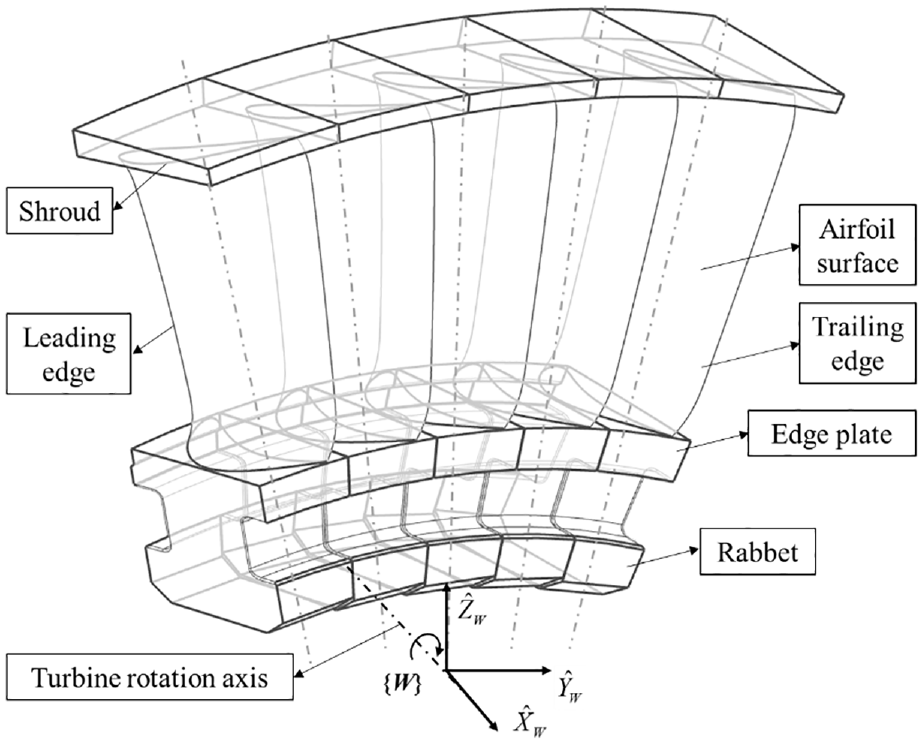
The features of the trubine blade.

In the process of blade grinding, several coordinate systems are involved, including the robot base coordinate system { B }, the robot flange coordinate system { F }, the workpiece coordinate system { W }, the mesurement coordinate system { M }, and the belt grinder coordinate system { H }. The calibration process is used for determining the relative relationship between those coordinate systems.

Calibration of the measurement coordiante system

Calibration for the 3D measurement equipment

As shown in Figure 3, the 3D measurement equipment consists of a motion platform and a 3D scanner fixed to it. The motion platform includes three mutually perpendicular translational axes and a rotational axis. The coordinate system of the 3D scanner is defined as { C }, and the coordinate system of the 3D measurement equipment is defined as { M }. Due to the assembly errors, it is difficult to ensure that the axes of { M } are completely parallel or perpendicular to the axes of { C }. The exact relationship between { C } and { M } needs to be determined by calibration.

Figure 3.

The 3D measurement equipment: (a) schematics and (b) calibration.

A fixed calibration ball is used for calibrating the relationship between { C } and { M }. It is assumed that the motion platform and the 3D scanner have been calibrated or compensated individually. The A-axis of the motion platform is always kept with a fixed angle. The three linear axes of the motion platform is moved so that the calibration ball is located on one side of the scanner field of view, and the point cloud data set {D₁} is obtained by scanning the calibration ball. Another point cloud data set {D₂} is sampled in the same way when the calibration ball is located on the other side.

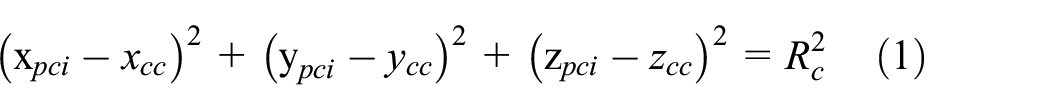
Assuming that the center of calibration ball is C_c , the radius of that is R_c, and any point in the spherical point cloud is P_ci , as shown in Figure 4. Two methods can be used for finding the value of C_c : one is NLS (Nonlinear Least Squares) and the other is RANSC (Random Sample Consensus). The RANSC results are always fluctuating due to its random nature. The NLS is adopted in this paper and a pass-through filter is applicated to select a suitable set of points. Any point P_ci (x_pci, y_pci, z_pci) in the point set satisfies equation (1), all points are substituted into equation (1) to form nonlinear equations, and the Levenberg-Marquardt method is used to obtain the solution of C_c (x_cc,y_cc,z_cc).

$${({\mathrm{x}}_{\mathrm{pci}}-x_{\mathrm{cc}})}^2+{({\mathrm{y}}_{\mathrm{pci}}-y_{\mathrm{cc}})}^2+{({\mathrm{z}}_{\mathrm{pci}}-z_{\mathrm{cc}})}^2=R_c^2$$

(1)

Figure 4.

Calculation algorithm of the calibration ball center.

Specifies a zero position for each axis of the measurement equipment and makes an initial movement to the zero position. It may be assumed that at the end of the initial movement, the origins of { M } and { C } are coincident, that is, ^M P _CORG  = (0, 0, 0) ^T or ^C P _MORG  = (0, 0, 0) ^T , and the fitted calibration sphere center is ^C P ₀. Then, the motion platform moves along ${\hat{X}}_M$ with distance dx, and the corresponding fitted calibration sphere center is ^C P ₁ after the movement. The movement along ${\hat{Z}}_M$ is conducted like that along ${\hat{X}}_M$ , and the corresponding variables are dz, ^C P₃. It is noted that the motion platform will return to the initial point before the movement along ${\hat{Z}}_M$ . The homogeneous transformation matrix from { M } and { C } is ${}_M^{C}T$

$$\begin{array}{c}{}_M^{C}T=\hfill \\ \left[\begin{array}{cccc}\mathrm{unit}({}^C{P}_1{}^C{P}_0)\hfill & \mathrm{unit}({}^C{P}_3{}^C{P}_0\times {}^C{P}_1{}^C{P}_0)\hfill & \mathrm{unit}({}^C{P}_3{}^{C}P)\hfill & {}^C{P}_{\mathrm{MORG}}\hfill \\ \multicolumn{1}{c}{0}& 0\hfill & 0\hfill & 1\hfill \end{array}\right]\hfill \end{array}$$

(2)

where unit() is the function to get unit vector. The homogeneous transformation matrix from { C } and { M } is denoted as ${}_C^{M}T$ which is the inverse matrix of ${}_M^{C}T$ . The space distance deviations of { M } and { C } are ignored.

Relationship between the coordinate systems of measurement and robot base _M^BT

As shown in Figure 5, a set of workpiece quick-change clamping system (WQCCS) is installed at the robot flange. The WQCCS has a fast pneumatic switcher. The switcher’s front end and rear end are fixedly connected to the robot flange and the blade fixture through adapter plates, respectively. The blade fixture can provide reliable positioning and clamping for various types of blades. The clamping and releasing of the switcher is pneumatically controlled. The nominal dimensions of WQCCS is known and real dimensions may contain errors. A calibration ball is fixed at the front end of the fast pneumatic switcher with unknown relative position.

Figure 5.

Workpiece quick-change clamping system (I. Calibration ball, II. Robot flange, III. Fast pneumatic switcher, IV. Adapter plate, V. Blade fixture, VI. Blade).

Rotation component of _M^BT

Keeping the calibration ball in the measurement range of { M }, the robot is moved to four positions as shown in Figure 6. The positions of the calibration ball center are denoted as C ₁, C ₂, C ₃, and C ₄, respectively. Those points are respectively represented as ^B C _i (i = 1, 2, 3, 4) and ^M C _i (i = 1, 2, 3, 4) in { B } and { M }, and satisfy the following relationship

$${}^B{C}_2{}^B{C}_1//{}^B\hat{X},{}^B{C}_3{}^B{C}_1//{}^B\hat{\mathrm{Y}},{}^B{C}_4{}^B{C}_1//{}^B\hat{\mathrm{Z}}$$

(3)

Figure 6.

The calibration ball positions for determining the rotation component of ${}_M^{B}T$ .

The unitization vectors of ${}^M{C}_2{}^M{C}_1$ , ${}^M{C}_3{}^M{C}_1$ , and ${}^M{C}_4{}^M{C}_1$ are denoted as ${}^{M}n$ , ${}^{M}o$ , and ${}^{M}a$ , respectively. Suppose ${}_M^{B}T=\left[\begin{array}{cc}{}_M^{B}R\hfill & {}^B{P}_{\mathrm{MORG}}\hfill \\ \multicolumn{1}{c}{0}& 1\hfill \end{array}\right]$ , then

$$\begin{array}{c}\multicolumn{1}{c}{{}_B^{M}R={\left({}_M^{B}R\right)}^{-1}=\mathrm{Rot}(\mathrm{Z},{}^M\alpha )\mathrm{Rot}(\mathrm{Y},{}^M\beta )\mathrm{Rot}(\mathrm{X},{}^M\gamma )}\\ =[{}^{M}n,{}^{M}o,{}^{M}a]\hfill \end{array}$$

(4)

where the function Rot(Z, ^M α) represents the transformation matrix of rotation ^M α around Z axis, and the definitions of Rot(Y, ^M β) and Rot(X, ^M γ) are similar. Due to errors, any two vectors of ${}^{M}n$ , ${}^{M}o$ , and ${}^{M}a$ are not strictly perpendicular. ^M α, ^M β, ^M γ, and ${}_M^{B}R$ can be solved by NLS according to equation (4).

Translation component of _M^BT

The robot was moved again to obtain four positions of the calibration ball center C ₅, C ₆, C ₇, and C ₈, with different robot postures (Figure 7). Suppose the transformation matrix from { F } to { B } ${}_F^B{T}_i=\left[\begin{array}{cc}{}_F^B{R}_i\hfill & {}^B{P}_{\mathrm{FORGi}}\hfill \\ \multicolumn{1}{c}{0}& 1\hfill \end{array}\right]$ at C _i+4 (i = 1, 2, 3, 4), then

$${}_F^B{R}_i{}^{F}C+{}^B{P}_{\mathrm{FORGi}}={}_M^{B}R{}^M{C}_{i+4}+{}^B{P}_{\mathrm{MORG}},i=1,2,3,4$$

(5)

where ${}_F^B{R}_i$ and ${}^B{P}_{\mathrm{FORGi}}$ are rotation and translation components of ${}_F^B{T}_i$ , ${}_F^B{T}_i$ is obtained from robot controller. ${}^{F}C$ is the positon of the calibration ball center in { F }. Equations (6) is consequently constructed.

$$\{\begin{array}{c}{}_M^{B}R({}^M{C}_6-{}^M{C}_5)=({}_F^B{R}_2-{}_F^B{R}_1){}^{F}C+({}^B{P}_{\mathrm{FORG}2}-{}^B{P}_{\mathrm{FORG}1})\hfill \\ \multicolumn{1}{c}{{}_M^{B}R({}^M{C}_7-{}^M{\mathrm{C}}_5)=({}_F^B{R}_3-{}_F^B{R}_1){}^{F}C+({}^B{P}_{\mathrm{FORG}3}-{}^B{P}_{\mathrm{FORG}1})}\\ \multicolumn{1}{c}{{}_M^{B}R({}^M{C}_8-{}^M{C}_5)=({}_F^B{R}_4-{}_F^B{R}_1){}^{F}C+({}^B{P}_{\mathrm{FORG}4}-{}^B{P}_{\mathrm{FORG}1})}\end{array}$$

(6)

${}^{F}C$ can be solved by equation (6), and ${}^B{P}_{\mathrm{MORG}}$ is also achieved when ${}^{F}C$ is substituted into equation (5).

Figure 7.

The calibration ball positions for determining translation component of ${}_M^{B}T$ .

Calibration of the workpiece coordinate system

Although the blade clamping error has been improved by the custom fixture, it may still be large at the far end (non-clamping end) of the blade due to the inherent drawbacks of single-end clamping of slender parts. The traditional method of directly determining the workpiece coordinate system through the fixture datum cannot meet the requirements of blade grinding accuracy. This paper uses a two-step method to determine the workpiece coordinate system: rough calibration and fine calibration.

Rough calibration of workpiece coordinate system

There are two ways to determine the initial workpiece coordinate system: (1) Calculate the initial value according to the dimensions and datums of the workpiece quick-change clamping system; (2) Measure the installed blade and its cooresponding CAD model for several feature points, and the initial value of { W } is solved by NLS. Those two ways are both suitable and the second way is illustrated in this paper. The positions of the feature points can be obtained by the four-point calibration method provided by the robot controller or directly selecting those points in the measuring point cloud.

As shown in Figure 8, the feature point P _i (i = 1, …, 13) is denoted as ^W P _i and ^F P _i in { W } and { F }, respectively. The transformation matrix from { W } to { F } is ${}_W^{F}T$ , and ${}_W^{F}T$ is represented as

$${}_W^{F}T=\left[\begin{array}{cc}\mathrm{Rot}(\mathrm{Z},{}^W\alpha )\mathrm{Rot}(\mathrm{Y},{}^W\beta )\mathrm{Rot}(\mathrm{X},{}^W\gamma )\hfill & {}^F{P}_{\mathrm{WORG}}\hfill \\ \multicolumn{1}{c}{0}& 1\hfill \end{array}\right]$$

(7)

where the function Rot(Z, ^W α) represents the transformation matrix of rotation ^W α around Z axis, and the definitions of Rot(Y, ^W β) and Rot(X, ^W γ) are similar. ${}^F{P}_{\mathrm{WORG}}$ is the origin position of { W } in { F }. Equations (8) can be established at P _i (i = 1, …, 13).

$$\{\begin{array}{c}{}^F{P}_1=\mathrm{Rot}(Z,{}^W\alpha )\mathrm{Rot}(Y,{}^W\beta )\mathrm{Rot}(X,{}^W\gamma ){}^W{P}_1+{}^F{P}_{\mathrm{WORG}}\hfill \\ \multicolumn{1}{c}{{}^F{P}_2=\mathrm{Rot}(Z,{}^W\alpha )\mathrm{Rot}(Y,{}^W\beta )\mathrm{Rot}(X,{}^W\gamma ){}^W{P}_2+{}^F{P}_{\mathrm{WORG}}}\\ \multicolumn{1}{c}{......}\\ \multicolumn{1}{c}{{}^F{P}_{13}=\mathrm{Rot}(Z,{}^W\alpha )\mathrm{Rot}(Y,{}^W\beta )\mathrm{Rot}(X,{}^W\gamma ){}^W{P}_{13}+{}^F{P}_{\mathrm{WORG}}}\end{array}$$

(8)

^W α, ^W β, ^W γ, and ${}^F{P}_{\mathrm{WORG}}$ are solved by least square according to equation (8), and the ${}_W^{F}T$ is consequently obtained according to equation (7).

Figure 8.

Blade feature points for { W } calibration.

Fine calibration of the workpiece coordinate system

The accuracy of the initial workpiece coordinate system is not high, which is mainly caused by the following reasons: (1) Asseembly or manufacturing error of the WQCCS; (2) Due to the material characteristics of the blade, it is difficult to produce an ideal sharp feature point; (3) The deviation in the point selection. In this paper, the rough calibration that only needs to be performed once for the same type of blade will provide a suitable initial value for the fine calibration of workpiece coordinate system.

The fine calibration of { W } is based on the scanning point data of blade multiple surfaces. Multiple scannings are required for a slender blade due to the limited measuring range of scanner. Solving { W } using the conventional point cloud algorithm requires stitching, registration, and other work. In the registration process, it is also necessary to discretize the CAD model surface. When there are a lot of point cloud data and iterative solutions such as ICP are used, the time-consuming of the algorithm will become unacceptable, and the registration accuracy is also difficult to guarantee due to the existence of a large number of non-blade surface points. A new method is used as follows in this paper.

Determination of surfaces for scanning

Since the motion accuracy of the 3D measurement equipment is much better than that of the robot, the blade remains stationary, and the scanning area of the blade is covered by the movement of the the 3D measurement equipment. While keeping the measurement accuracy, the scanned surfaces should be as many as possible in each scan and the number of measurements should be as few as possible.

As shown in Figure 9, the blade is scanned twice by moving the 3D scanner. The first scan area is located at the edge plate, involving the surface S₁ (P₈P₉P₁₀), S₂ (P₉P₁₀P₁₃P₁₂), and S₃ (P₈P₉P₁₂P₁₁); the second scan is located at the shroud, involving surface S₄ (P₁P₂P₃P₄), S₅ (P₁P₂P₆P₅), and S₆ (P₂P₃P₇P₆). When scanning, the ${\hat{Z}}_C$ of scanner is perpendicular to the paper in Figure 9, and the target scanning area is located in the center of the field of view.

Figure 9.

The target surfaces for scanning on the blade.

The angle between the surface S₂ and S₃, and that between the surface S₅ and S₆ are obtuse angles, which is beneficial to ensure that all target surfaces in the scanning area maintain a reasonable light angle for the scanner. The two scanned surfaces are distributed at both ends of the blade, which is beneficial to control the blade deflection error. The points on the surface S₂, S₃, S₅, and S₆ are mainly used to constrain the position of the blade in the XY-plane of the { W }, and the movement along ${\hat{Z}}_W$ is constrained by the points on the surface S₁ and S₄.

Point cloud data extraction on scanned surfaces

When using a 3D scanner to scan the blade, it is inevitable to introduce some non-blade surface points, such as points on the fixture, these points need to be eliminated. In addition, the scanning point cloud may come from multiple surfaces on the blade, and it is difficult to distinguish the target surface.Therefore, this paper uses a local space related to the surface type and boundary to filter out the discrete points on the corresponding surface, and discusses separately according to the characteristics of the surface type and boundary.

According to the blade CAD model, it can be seen that the surface S₁ and S₄ are cylindrical surfaces, while the surface S₅, S₆, S₂, and S₃ are planes. Since the area of surface S₁ which can be scanned is very small, the points on surface S₁ will not be used in the later algorithm.

The extraction of scanning points on the cylindrical surface S₄ is shown in Figure 10, and the situation of the surface S₃ is similar. In { W }, the cylindrical surface S₅ can be expressed in the form of parameters $S_{\mathrm{cyl}}(u,v)$ in equation (9).

$$\begin{array}{c}\multicolumn{1}{c}{S_{\mathrm{cyl}}(u,v)=v{}^W{\hat{Z}}_{\mathrm{CY}}+R_{\mathrm{cyl}}\cos \left(u\right){}^W{\hat{X}}_{\mathrm{CY}}+R_{\mathrm{cyl}}\sin \left(u\right){}^W{\hat{Y}}_{\mathrm{CY}}}\\ +{}^W{P}_{\mathrm{CYORG}}\hfill \end{array}$$

(9)

where R_cyl is the cylindrical radius, ${}^W{P}_{\mathrm{CYORG}}$ , ${\hat{X}}_{\mathrm{CY}}$ , ${\hat{Y}}_{\mathrm{CY}}$ , and ${\hat{Z}}_{\mathrm{CY}}$ are the coordinate system origin, X-axis, Y-axis, and Z-axis of the cylindrical surface in { W }. The boundary P₁P₂ and P₃P₄ are in a plane perpendicular to ${\hat{X}}_W$ , and both are part of cylindrical arcs. The boundary P₁P₄ and P₂P₃ are the intersection of plane and cylinder. Due to the error of the initial value of { W } and the possible accuracy distortion of scanning points on the boundary, this paper uses the following method to construct the local filtering area to ensure that the points on the adjacent surface are not mixed into the point cloud of the target surface. First, shrink all boundaries inward in the cylindrical surface S₄ with δ₁, as shown in Figure 10(a), and the cylindrical area after shrinkage is P′₁P′₂P′₃P′₄. Then, as shown in Figure 10(b), expand the cylindrical surface P′₁P′₂P′₃P′₄ along the positive and negative normal direction with δ_h1, forming the upper and lower boundary interfaces, and the space between those two boundary surfaces is the local filter space.

Figure 10.

Filter box for cylinder surface: (a) shrink on the surface and (b) expand along surface normal direction.

The upper and lower boundaries of plane S₅ and S₃ are two concentric arcs (the arcs with the same center), the left and right boundaries are straight lines. The plane is parameterized as

$$S_{\mathrm{plane}}(u,v)=u{}^W{\hat{X}}_{\mathrm{PL}}+v{}^W{\hat{Y}}_{\mathrm{PL}}+{}^W{P}_{\mathrm{PLORG}}$$

(10)

where ${}^W{P}_{\mathrm{PLORG}}$ , ${\hat{X}}_{\mathrm{PL}}$ , and ${\hat{Y}}_{\mathrm{PL}}$ are the coordinate system origin, X-axis and Y-axis of the plane in { W }. Figure 11(a) shows the processing of the plane S₅, and that of the plane S₃ is similar. As with the cylindrical treatment process, the boundary is shrunk inward in the plane S₅ with δ₂. Translate the result plane P″₁P″₂P′₆P′₅ along the positive and negative normal directions with δ_h2, respectively, to obtain the front and rear boundary planes, and the space between those two boundary planes is the local filter space.

Figure 11.

Filter box for plane surface with arc boundaries: (a) shrink on the surface and (b) expand along surface normal.

The upper boundaries of the plane S₆ and S₂ are the intersection curves of the plane and the cylinder. After analyzing all the blade models to be processed, it is found that the boundary P₂P₃ or P₉P₁₀ are relatively straight. For convenience, the curve P₂P₃ or P₉P₁₀ is directly processed as a straight line. The plane S₂ only takes the quadrilateral area surrounded by the four corners, and the rest is difficult to be scanned due to fixture occlusion. As shown in Figure 12, similar to the cylindrical processing method, the boundary is shrunk inward by δ₃ on the plane S ₂, and the result plane P′₉P′₁₀P′₁₃P′₁₂ is translated along the positive and negative directions of the plane normal by δ_h3, respectively. The space between these front and rear boundary planes is the local filtering space. The processing of the plane S₆ is the same as that of the plane S₂.

Figure 12.

Filter box for plane surface with straight ine boundaries: (a) offset on the surface and (b) offset along surface normal direction.

Solve the transformation matrix for {W}

Traditional ICP-centric algorithms are difficult to meet the precision and efficiency requirements of blade grinding, especially when the number of scanned points increases. The CAD model of workpiece generally exists while dealing with a machining problem, and the analytical expressions of each surface can be obtained. Therefore, the optimal target is set as the minimum sum of squares of the errors between the measurement point cloud and the model surfaces of blade in this paper. The error here is no longer the distance of point pair as in ICP-centric algorithms, but the distance between analytical model surface and corresponding filtered point cloud. The optimal transformation matrix of { W } is expressed as follows.

$${}_W^F{T}^{*}=\underset{{}_W^{F}T}{\arg }min\sum _{i=0}^n{d}_{\mathrm{SURi}}^2$$

(11)

where $d_{\mathrm{SURi}}$ is the point-surface distance. The surface can be a plane or a cylinder, and $d_{\mathrm{SURi}}=d_{\mathrm{PLi}}$ , $d_{\mathrm{SURi}}=d_{\mathrm{CYi}}$ , respectively. $d_{\mathrm{PLi}}$ , $d_{\mathrm{CYi}}$ is defined as equations (12) and (13), respectively.

$$d_{\mathrm{PLi}}=({}^W{P}_{\mathrm{PLi}}-{}^W{P}_{\mathrm{PLORG}})·{}^W{\hat{Z}}_{\mathrm{plane}}$$

(12)

$$\begin{array}{c}{d}_{\mathrm{CYLi}}=\hfill \\ \Vert ({}^W{P}_{\mathrm{CYLi}}-{}^W{P}_{\mathrm{CYORG}})-(({}^W{P}_{\mathrm{CYLi}}-{}^W{P}_{\mathrm{CYORG}})·{}^W{\hat{Z}}_{\mathrm{plane}}){}^W{\hat{Z}}_{\mathrm{plane}}\Vert \hfill \\ -R_{\mathrm{cyl}}\hfill \end{array}$$

(13)

The solution of the optimization problem of equation (11) is equivalent to the least square solution of $d_{\mathrm{SURi}}=0$ .

Calibration of the tool coordination system

The schematic model of the abrasive belt grinder is shown in Figure 13, which mainly includes the base, the floating force control grinding unit, and the belt driving and tensioning unit. The floating force control grinding unit consists of a floating grinding head, an air cylinder, a force sensor, and an angle sensor. The belt driving and tensioning unit is not shown in the schematic model. Under grinding force, the contact wheel at the front end of the grinding head rotates together with other parts around the rotation axis. The cylinder pressure is maintained at the specified value to achive a constant grinding contact force. The force sensor is used to monitor the actual output force of the cylinder. The rotation angle of the grinding head is recorded by the angle sensor.

Figure 13.

The structure of abrasive belt grinder.

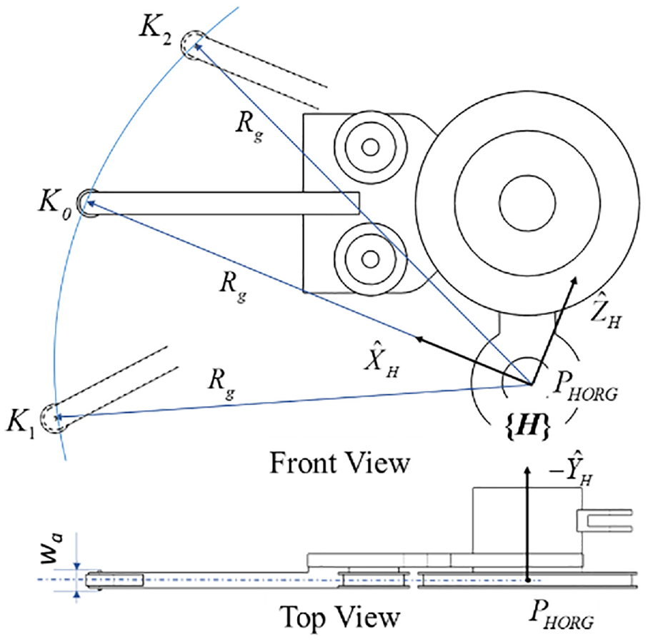
The coordinate system of the belt grinder is marked as { H } and is fixed to the grinder base. As shown in Figure 14, the ${\hat{Y}}_H$ of { H } is consistent with the rotation axis of the floating grinding head. The ${\hat{Z}}_H{\hat{X}}_H$ -plane passes through the center of the contact wheel while the origin of { H } $P_{\mathrm{HORG}}$ is also determined. The position of contact wheel center is denoted as K₀ when the value of angle sensor is zero, and the direction of ${\hat{X}}_H$ is the same as that of $P_{\mathrm{HORG}}{K}_0$ . ${\hat{\mathrm{Z}}}_H={\hat{X}}_H\times {\hat{Y}}_H$ .

Figure 14.

The coordinate system of abrasive belt grinder.

The positions of the contact wheel center with the angle sensor values ${}^H{\alpha }_1$ , ${}^H{\alpha }_2$ are denoted as $K_1$ , $K_2$ , respectively. The ${\hat{Z}}_H{\hat{X}}_H$ -plane is fitted by points $K_0$ , $K_1$ , $K_2$ using SVD (Singular Value Decomposition) algorithm. $P_{\mathrm{HORG}}(x_{\mathrm{HORG}},y_{\mathrm{HORG}},z_{\mathrm{HORG}})$ is in this fitted plane, and satisfy equation (14).

$$a{x}_{\mathrm{HORG}}+b{y}_{\mathrm{HORG}}+c{z}_{\mathrm{HORG}}=d$$

(14)

where a, b, c, d are plane coefficients. The distance between the rotation axes of the floating grinding head and the contact wheel is denoted as R_g, then

$$\{\begin{array}{c}\Vert K_0{P}_{\mathrm{HORG}}\Vert =R_g\hfill \\ \multicolumn{1}{c}{\Vert K_1{P}_{\mathrm{HORG}}\Vert =R_g}\\ \multicolumn{1}{c}{\Vert K_2{P}_{\mathrm{HORG}}\Vert =R_g}\\ \multicolumn{1}{c}{K_0{P}_{\mathrm{HORG}}·K_1{P}_{\mathrm{HORG}}=R_g^2\cos ({}^H{\alpha }_1-0)}\\ \multicolumn{1}{c}{K_0{P}_{\mathrm{HORG}}·K_2{P}_{\mathrm{HORG}}=R_g^2\cos ({}^H{\alpha }_2-0)}\end{array}$$

(15)

$P_{\mathrm{HORG}}(x_{\mathrm{HORG}},y_{\mathrm{HORG}},z_{\mathrm{HORG}})$ contains two unknown components considering equation (14). Although the theoretical value of R_g can be measured by the CAD model, it is not reliable due to the installation allowance of the rod where the contact wheel is located, and R_g is still regarded as unknown. Therefore, the values of $P_{\mathrm{HORG}}$ and R_g can be solved by NLS method according to equation (15). Similar to K₀, K₁, K₂, increasing the sampling points number of the contact wheel center and expanding the rotation angle scope of the floating grinding head are beneficial to obtain a more accurate and stable solution.

$${\hat{X}}_H=K_0{P}_{\mathrm{HORG}}/\Vert K_0{P}_{\mathrm{HORG}}\Vert$$

(16)

$${\hat{Y}}_H=\pm [a,b,c{]}^T/\mathrm{sqrt}(a^2+b^2+c^2)$$

(17)

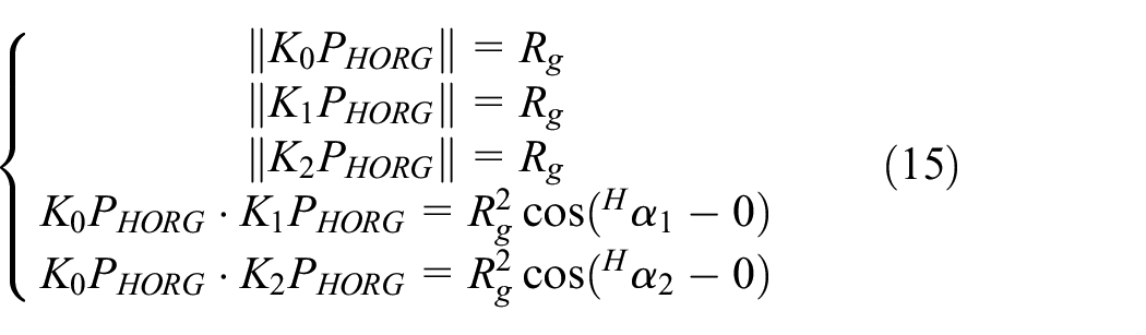
where the sign of ${\hat{Y}}_H$ is determined by $K_1{P}_{\mathrm{HORG}}\times K_2{P}_{\mathrm{HORG}}$ .

It is noted that in this paper, the measurement of K₀, K₁, K₂ is done by a stylus fixed to the robot flange. The stylus head position in { F } is achieved by the built-in four-point calibration method of the robot. When measuring K₀, K₁, K₂, the robot is moved to make the stylus head coincide with the side center of the contact wheel shaft, and the positions of sylus head in { B } are recorded. The length of the contact wheel shaft is denoted as w_a, as shown in Figure 14. Therefore, the calculated $P_{\mathrm{HORG}}$ should be translated along $-{\hat{Y}}_H$ with the value −w_a/2 using the above measurement scheme.

Error surface construction and error compesation

Various errors are involved in the calibration process of the grinding system, including robot positioning error, scanner measurement error, stylus calibration error, mechanical error of belt grinder, etc. In addition, the blade airfoil surface formed in the previous process of grinding always has deviation from that in the CAD model. The ideal processing effect cannot be obtained directly using the calibration results. The above error factors, including the shape error of the blade airfoil surface, have good repeatability under mass production conditions. Therefore, compensating for the blade error will significantly improve the precision of the robot grinding trajectory.

Figure 15 shows the relationship between the airfoil section and the floating grinding head during grinding. The contact wheel is in contact with the airfoil surface at one point (if it is a line contact, the midpoint of the contact line is taken), and this point on the contact wheel is denoted as $Q_c$ regardless of the rotation of the contact wheel. The angular position of the point on the contact wheel remains unchanged. The contact wheel center is denoted as K_c. In order to ensure that the normal error of the airfoil surface at the contact point has the maximum sensitivity to the rotation angle change of the floating grinding head, this paper takes $Q_c{K}_c\perp K_c{P}_{\mathrm{HORG}}$ . The contact point on the airfoil surface is denoted as $Q_{i,j}$ , the normal vector of the airfoil surface at $Q_{i,j}$ is ${\hat{n}}_{i,j}$ , and the tangent vector of the trajectory curve is ${\hat{T}}_{i,j}$ . Assuming that the actual contact point caused by blade errors is $Q_{i,j}^{\prime }$ , then the normal error $e_{i,j}^n$ at $Q_{i,j}$ can be expressed as

$$e_{i,j}^n=(Q_{i,j}^{\prime }-Q_{i,j})•{\hat{n}}_{i,j}=\mathrm{\Delta }{Q}_{i,j}•{\hat{n}}_{i,j}$$

(18)

The angle change of the floating grinding head caused by $e_{i,j}^n$ is denoted as $e_{i,j}^a$ , and

$$e_{i,j}^n\approx e_{i,j}^a\Vert K_c-P_{\mathrm{HORG}}\Vert$$

(19)

$e_{i,j}^a$ is measured by the angle sensor. Combining equations (18) and (19), it is difficult to obtain $Q_{i,j}^{\prime }$ . $Q_{i,j}^{\prime }$ has little effect on grinding accuracy in the direction of ${\hat{T}}_{i,j}$ and ${\hat{n}}_{i,j}\times {\hat{T}}_{i,j}$ , while it has great influence in the direction of ${\hat{n}}_{i,j}$ . Therefore, the projection point of $Q_{i,j}^{\prime }$ on the ${\hat{n}}_{i,j}$ denoted by $Q_{i,j}^n$ is solved instead.

$$Q_{i,j}^n=Q_{i,j}+e_{i,j}^n{\hat{n}}_{i,j}$$

(20)

The blade airfoil surface is defined as B-spline surface S (u, v) in the blade CAD model

$$S(u,v)=\sum _{i=0}^n\sum _{j=0}^m{N}_{i,p}\left(u\right)N_{j,q}\left(v\right)P_{i,j}$$

(21)

where $N_{i,p}\left(u\right)$ and $N_{j,q}\left(v\right)$ are B-spline base functions, their degrees are p and q, respectively. $P_{i,j}$ is control point and knot vectors are U and V , respectively. The v-isoparametric curve S(u, v_const) on S (u, v) is in the ${\hat{X}}_W{\hat{Y}}_W$ -plane of { W }, and the u-isoparametric curve S(u_const, v) on S (u, v) roughly follows the direction ${\hat{Z}}_W$ . The definition domains of u and v are [u_min, u_max], [v_min, v_max], respectively. The definition domains corresponding to the processing or measuring area are [u′_min, u′_max] ⊆ [u_min, u_max], [v′_min, v′_max] ⊆ [v_min, v_max], respectively. The surface is divided into n′ parts in the u-direction according to the constraints of chord error and step length in the processing or measuring area. The curvature in the v-direction changes little and the surface is divided into m′ parts at equal v intervals. Any combination of u and v is recorded as [u_i, v_j], i = 0, 1, 2 …, n′, j = 0, 1, 2, …, m′. The corresponding point of [u_i, v_j] on S (u, v) is $Q_{i,j}$ , and the normal error $e^n(u,v)$ can be expressed as

$$e^n(u,v)=\sum _{i=0}^{n\prime }\sum _{j=0}^{m\prime }{N}_{i,p}\left(u_i\right)N_{j,q}\left(v_j\right)e_{i,j}^c$$

(22)

where $e_{i,j}^c$ is control point of one-dimension, and equation (22) is also called error surface. $e^n(u_i,v_i)=e_{i,j}^n$ is established at i = 0, 1, 2 …, n′, j = 0, 1, 2, …, m′, forming (n′ + 1) × (m′ + 1) equations, and $e_{i,j}^c$ can be solved.

Figure 15.

Error analysis of the balde during grinding.

As shown in Figure 16, there are generally two ways to plan the trajectory of the airfoil surface grinding: (a) transverse processing and (b) longitudinal processing. The trajectories are v-isoparametric and u-isoparametric curves during transverse and longitudinal grinding, respectively. The interval between two adjacent trajectories does not change much during transverse machining, but if there is an error in the normal direction of the contact wheel and the airfoil surface, it is easy to generate banded pattern on the ground surface. Longitudinal grinding can control banded pattern easily, but the interval between adjacent trajectory varies greatly from the edge plate to the shroud, which affects the processing efficiency.

Figure 16.

Trajectory planning methods for robotic belt grinding: (a) transverse grinding and (b) longitudinal grinding.

Assuming that the transverse grinding is adopted, the theoretical trajectory curve R_k(u) is expressed as

$$R_k\left(u\right)=S(u,v_k^t)=\sum _{i=0}^n\sum _{j=0}^m{N}_{i,p}\left(u\right)N_{j,q}\left(v_k^t\right)P_{i,j}$$

(23)

The trajectory error ΔR_k(u) is expressed as

$$\mathrm{\Delta }{R}_k\left(u\right)=e^n(u,v_k^t)·\hat{n}(u,v_k^t)$$

(24)

where, $\hat{n}(u,v_k^t)$ is the normal vector of airfoil surface S (u,v) at $(u,v_k^t)$ . The actual trajectory is R_k(u)+ΔR_k(u). The above method of constructing error surface before trajectory planning can ensure that trajectory planning is independent from specific measurement points. When the interval between trajectories needs to be adjusted in blade rough and finish machining, it can be adjusted conveniently without being limited by the positions of specific measuring points.

Simulation and verification

The calibration of the measurement equipment

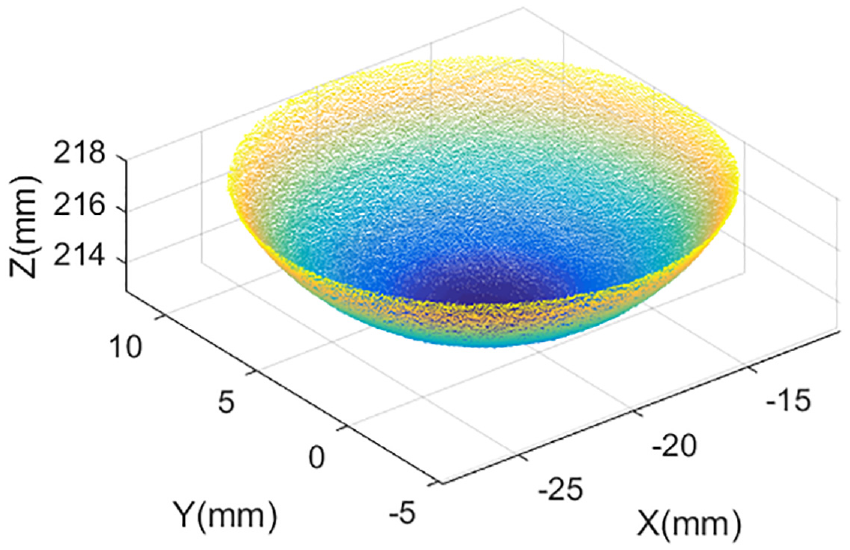
The scanner model used in this article is PhoXi 3D Scanner XS (scanning area at sweet spot: 118 × 78 mm, point to point distance: 0.055 mm, calibration accuracy (1σ): 0.035 mm). The positioning accuracy of each linear axis is less than 2 μm, and the rotary axis is kept with a fixed angle. In this paper, a matt ceramic calibration ball with a diameter of 19.988 mm is used. The scaned data of the calibration ball with a simple filter z < 218 mm is shown in Figure 17. The diameter of the calibration ball obtained by equation (1) is 20.020 mm, with an error of 0.032 mm, which is acceptable compared with the calibration accuracy (1σ) of the scanner. The spherical center coordinates are (−19.600, 3.458, 222.921) mm.

Figure 17.

The scaned data of the calibration ball with a simple filter z < 218 mm.

There are angle deviations between corresponding axes of { M } and { C } and the simulation data are provided as dx = 110 mm, dz = 55mm, ^C P ₀ = (−55.0, −27.5, 0.0) mm, ^C P ₁ = (54.0, −27.0, 0.5) mm, ^C P ₂ = (−54.0, 28.0, −0.5) mm. The result of ${}_C^{M}T$ is ${}_C^{M}T=\left[\begin{array}{cccc}0.999979\hfill & 0.004587\hfill & 0.004587\hfill & 0\hfill \\ \multicolumn{1}{c}{0.004629}& -0.009092\hfill & -0.999948\hfill & 0\hfill \\ \multicolumn{1}{c}{0.018014}& 0.999797\hfill & -0.009007\hfill & 0\hfill \\ \multicolumn{1}{c}{0}& 0\hfill & 0\hfill & 1\hfill \end{array}\right]$ .

The calibration of {M}

The values of ^M α, ^M β, ^M γ, ^B P_MORG, ^F C given for simulation are listed in the row SV of Table 1. Other simulated values are given as follows, ^M C₁ = (20.006, 20.000, 19.994) mm, ^M C₂ = (169.960, 22.618, 17.376) mm, ^M C₃ = (17.434, 169.955, 22.611) mm, ^M C₄ = (22.669, 17.428, 169.948) mm, ^M C₅ = (20.006, 20.000, 19.994) mm, ^M C₆ = (149.954, 2.617, −2.618) mm, ^M C₇ = (−2.572, 149.955, 2.617) mm, ^M C₈ = (2.663, −2.572, 149.954) mm, ^B P_FORG1 = (−1246.000, −1510.000, 965.000) mm, ^B P_FORG2 = (−1116.000, −1527.577, 959.514) mm, ^B P_FORG3 = (−1266.000, −1383.678, 930.752) mm, ^B P_FORG4 = (−1251.292, −1523.132, 1095.000) mm, ${}_F^B{R}_1$  = Rot(Y, π/2), ${}_F^B{R}_2$  = Rot(Y, π/2) Rot(X, 5/180*π), ${}_F^B{R}_3$  = Rot(Y, π/2) Rot(X, −5/180*π), ${}_F^B{R}_4$  = Rot(Y, π/2) Rot(Z, 5/180*π). Considering measurement and robot positioning errors, an error item with normal distribution N (0, 0.06²) is imposed to ^M C_i, i = 1, …, 8. The calibration results of { M } is listed in the row CV of Table 1. The row DEV shows deviations between SV and CV. Some components of the deviations are significantly larger than the given error item N (0, 0.06²), and this also shows the necessity of error compensation later.

Table 1.

The calibration results of { M }.

	M α (°)	M β (°)	M γ (°)	B PMORG (mm)	F C (mm)
SV	1.000	1.000	1.000	−1180.000, −1695.000, 980.000	−35.000, −165.000, 86.000
CV	1.015	0.956	0.971	−1179.933, −1695.429, 980.051	−35.046, −165.445, 86.088
DEV	0.015	−0.044	−0.029	0.067, −0.429, 0.051	−0.046, −0.445, 0.088

The calibration of the {W}

The rough calibration is conducted first. Taking the blade (DR95.23.02.23) as an example, five points P ₅, P ₈, P ₇, P ₁₀, and P ₄ shown in Figure 8 are selected. The coordinate values of those points in CAD model are (38.000, 58.391, 635.832) mm, (36.000, 45.636, 439.638) mm, (−36.000, −56.914, 629.610) mm, (−34.000, −44.534, 439.751) mm, (−36.000, 18.167, 649.246) mm, respectively. The correspoinding coordinate values obtained by the robot built-in four-point calibration method are (69.841, −46.634, 677.333) mm, (54.620, −51.967, 481.377) mm, (−46.035, 26.351, 669.857) mm, (−36.017, 17.416, 480.058)  mm, (29.284, 27.554, 688.521) mm, respectively. Solve equation (8), and obtian ^W α = −89.609°, ^W β = −2.113°, ^W γ = −0.731° and ${}^F{P}_{\mathrm{WORG}}$  = (3.245, −32.528, 41.328) mm.

Then the fine calibration is conducted and simulation is adopted to verify. The blade CAD model is discretized at 1.0 mm spacing, as shown in Figure 18(a). The raw data from scanner is denser, but is generally downsampled to increase computational speed. The simulated measurement error of N (0, 0.035²) is superimposed on the normal direction of the surface. It is assumed that the actual values of ^W α, ^W β, ^W γ, and ${}^F{P}_{\mathrm{WORG}}$ are −90°, 0°, 0° and (3, −32, 41) mm for simulation according to the initial calibration value of ${}_W^{F}T$ , respectively. The simulated point cloud of the blade is then obtained under { F }. The virtual scans are conducted to cover the surfaces shown in Figure 9. The corresponding point clouds of those five scaned surfaces are seperated with filter paramenters δ_i = 2 mm, δ_h2 = 2 mm, i = 1, 2, 3, as shown in Figure 18(b).

Figure 18.

The blade point cloude: (a) original data and (b) filtered data.

The optimal value ${}_W^F{T}^{*}$ of the transformation matrix of { W } is obtained according to equation (11). The optimal values of ^W α^*, ^W β^*, ^W γ^*, and ${}^F{P}_{\mathrm{WORG}}^{*}$ are listed in the row CV of Table 2. The deviations (row DEV) between simulated values (row SV) and calculated values (row CV) are very small. The fine calibration algorithm has good anti-interference ability to the measurement error.

Table 2.

The fine calibration results of { W }.

	W α (°)	W β (°)	W γ (°)	F PWORG (mm)	Running time (s)
SV	−90.000000	0.000000	0.000000	(3.000, −32.000, 41.000)	0.061
CV	−89.998722	0.000122	−0.000116	(3.000, −32.000, 41.000)
DEV	0.001278	−0.000122	−0.000116	(0.000, 0.000, 0.000)

In order to compare with ICP algorithm, this paper selects surface S2–S6 in Figure 9, uses 0.55 mm spacing, and applies errors N (0,0.035²) in the normal direction of each point to generate simulation scanning data. Blade CAD model is also converted into point cloud model with 0.5 mm spacing. The ICP registration method in Computer Vision ToolBox of Matlab 2021b is used to solve the pose transformation from the scanned point cloud to that of the whole blade. The results are shown in Table 3.

Table 3.

The fine calibration results of { W } by ICP algorithm.

	W α (°)	W β (°)	W γ (°)	F PWORG (mm)	Running time (s)
SV	−90.000000	0.000000	0.000000	(3.000, −32.000, 41.000)	1.516
CV	−90.415221	−0.066865	0.040444	(3.032, −32.275, 41.008)
DEV	−0.415221	−0.066865	0.040444	(0.032, −0.275, 0.008)

The results in Tables 2 and 3 shows that although ICP algorithm uses smaller point to point spacing, the calibration error is larger and cannot meet the grinding requirements. Increasing the point cloud density can improve the accuracy of ICP calibration result, but the algorithm running time will be significantly extended. Running in the same computer with a CPU E5-2667, the consumption time of ICP algorithm is about 25 times of that the algorithm proposed in this paper.

The calibration of {H}

Firstly, the simulation conditions are given. The origin of { H } in { B } ( ${}^B{\mathit{P}}_{\mathrm{HORG}}$ ) is (1420, 1210, 940) mm, the length of contact wheel shaft is w_a = 12 mm, and $\Vert {}^B{K_c}^B{P}_{\mathrm{HORG}}\Vert =\sqrt{{390}^2+{160}^2}$  = 421.545 mm. As shown in Figures 1 and 14, the orientation of { H } in { B } is Rot(Z, 135) Rot(Y, −22.306205), and ${}^H{\alpha }_0$  = 0, ${}^H{\alpha }_1$  = 30°, ${}^H{\alpha }_2$  = −30°. The simulated values of ${}^B{K}_0$ , ${}^B{K}_1$ , ${}^B{K}_2$ are calculated as (1144.228, 1485.772, 1100.000) mm, (1124.606, 1505.394, 883.564) mm, (1237.743, 1392.257, 1273.564) mm, respectively.

Then the coefficients of fitted plane where ${}^B{K}_0$ , ${}^B{K}_1$ , and ${}^B{K}_2$ lie is calculated using equation (14), a = −0.707107, b = −0.707107, c = 0.000000, d = −1859.690835. Using equation (15), ${}^B{P}_{\mathrm{HORG}}$  = (1420.000, 1210.000, 940.000), R_g = 425.545, ${}^B{\hat{X}}_H$  = (−0.654193, 0.654193, 0.379556), ${}^B{\hat{Y}}_H$  = (0.707107, 0.707107, 0.000000) are solved. ${}^B{P}_{\mathrm{HORG}}$ and R_g have no deviation from their simulated values.

Error airfoil surface construction and error compensation

Two types of simulated errors are given in this paper, one is the shape error of the blade airfoil surface, and the other is the pose error caused by the error factors of the grinding system such as robot positioning error. The shape error is simulated by a cosine distribution along the airfoil surface parameter v, and can be approximately expressed as E_s(v) = 0.5 cos(4πv), v∈[0, 1].

The pose error E_r is simulated to be offset by 0.5 mm in the ${\hat{Y}}_W$ direction and rotated by 0.1° around ${\hat{X}}_W$ . $E_r\left(u,v\right)=(\mathrm{Rot}\left(X,0.1/180\ast \pi \right)·\mathbf{S}\left(u,v\right)+{\left(0,0.05,0\right)}^T-\mathbf{S}\left(u,v\right))·{\widehat{\mathbf{n}}}_w\left(u,v\right)$ , ${\hat{\mathbf{n}}}_w(u,v)$ is the normal vector of S (u, v) at (u, v). The distribution of the composite error E_s+E_r of the airfoil surface is shown in Figure 19.

Figure 19.

Simulated errors of blade airfoil surface.

Plan measurement points

According to the process arrangement, the trailing edge area and the transition area of the airfoil surface near shroud and edge plate will be processed manually after robot grinding due to interference or too small curvature radius. The measuring and grinding range is $v\in$ [0.028170, 0.946634], $u\in$ [0.05000, 0.950000]. The measurement trajectories are formed by the intersection of the airfoil surface and a series of planes perpendicular to ${\hat{Z}}_W$ , and, that is, several v-isoparametric curves. The interval between adjacent planes is set to 2 mm. The curvature changes greatly along a v-isoparametric curve and it is necessary to adjust measurement point density according to the curvature value. The constraints of chord error (≤0.001 mm) and adjacent point distance (≤10 mm) are imposed and the resultant sampling points are shown in Figure 20.

Figure 20.

Points on the airfoil surface for measurement.

Construct error surface

According to the sampling points planned in Figure 20, the airfoil surface is scanned line by line according to the blade CAD model and the calibrated pose, and the measurement results are recorded online. As shown in Figure 21, the error of the airfoil surface sampling area is within the interval [−1, 1] mm.

Figure 21.

Errors of blade airfoil surface at sample points.

According to equation (22), the error surface e ⁿ (u, v) is obtained by interpolation. The cubic B-spline basis functions are used for both u and v, the number of control points n′+1 = 129, m′+1 = 40. The first and last of node control vectors U and V adopt 4-repetition style. Figure 22 shows the deviations between the error surface e ⁿ (u, v) and the simulated one (Figure 19). As can be seen from Figure 22, the deviations are larger at the leading edge and fluctuate at both ends of u-isoparametric curves. The error of the leading edge varies sharply, resulting in a large fitting error of e ⁿ (u, v) in this part. The fluctuation at both ends of u-isoparametric curves may caused by mismatch of end conditions. The overall deviations in Figure 22 are within [−2.5, 2.5] μm, which fully meets the requirements compared with scanner accuracy and robot positioning accuracy.

Figure 22.

Deviations between interpolation error surface and simulated error surface.

Compesate trajectory errors

According to equations (23) and (24), along the grinding path, the compensation amount ΔR_k(u) is calculated. In Figure 23, traj-err-1–traj-err-6 are the trajectories when v = 0.02817023, 0.21657314, 0.40497606, 0.59337898, 0.7817819, and 0.94663445 respectively during transverse grinding.

Figure 23.

Trajectory errors for compesation.

Conclusions

1. The scanner-based calibration method proposed in this paper provides a complete solution for the calibration of the robotic abrasive belt grinding system. The scanner range is expanded by the precision motion platform. The point recognition accuracy is imporved by the calibration ball. The relationships among robot base coordiante system { B }, measurement coordinate system { M }, blade workpiece coordiante system { W }, belt grinder tool coordiante system { H } are established.

2. The calibration method of { W } based on scaned point cloud and CAD model proposed in this paper realizes the rapid segmentation of point cloud. The distance functions from discrete points to their corresponding parametric surfaces are established, and the transformation matrix of { W } is obtained by NLS. This method makes full use of the characteristics of parametric surfaces and avoids the errors caused by surface discretization. Compared with ICP-centric algorithms, the efficiency is greatly improved, and the online calibration will not affect the production takt in mass production.

3. The construction and compensation method of blade error surface proposed in this paper eliminates the influence of most error factors in the system, such as robot absolute positioning error, calibration error, workpiece shape error, etc., and improves the grinding accuracy. The error surface is interpolated by error points which are converted from the rotation angles of the floating grinding head, and it has the same u and v parameters as the designed airfoil surface, which is convenient for direct superposition and can be reused.