Sage Journals: Discover world-class research

Abstract

This article presents an investigation for the secondary flow characteristics and associated pressure loss in fluid flow through helically coiled pipe. Computational fluid dynamics is employed to analyze the pipe flow with various geometries, and the accuracy of the numerical methodology is validated by conducting corresponding experiments. The analysis performs a detailed parametric study involving the pressure loss, the secondary vortex motion, and the secondary vortex intensity for a range of coil diameters (D; ranging from 300 to 3000 mm) and pipe diameters (d; ranging from 50 to 90 mm). The pipe flow develops to a stable state with increase in coil diameter, while an increase in pipe diameter delays this development. Then, the secondary flow characteristics are analyzed to explore the pressure loss mechanism. The distorted streamline of secondary vortices and the enlarged deflection angle of secondary vortices are both factors contributing to the enhanced pressure loss. Furthermore, the effects of pipe flow development on the following flow characteristics such as the turbulence dissipation rate and the secondary vortex intensity are revealed. These characteristics all distribute regularly and reach lower values when pipe flow begins to a stable state.

Keywords

Secondary vortex helical pipe pressure loss secondary flow characteristics computational fluid dynamics

Introduction

Fluid flow through helically coiled pipe is a common occurrence in a vast range of agricultural and industrial applications, such as farm irrigation, wet dedusting, and heat exchangers. In helically coiled pipe, the secondary flow induced by the bend hinders the flow, goes smoothly along the main flow direction, and appears as a pair of counter-rotating vortices in the cross-section normal to the primary flow direction. Therefore, the helically coiled pipe generates more pressure loss in overcoming the minor (secondary) flow.

Many studies have reported on the influence of coil parameters on the pressure loss for helically coiled pipes. Ghobadi and Muzychka¹ developed an asymptotic model based on the experimental results to predict the pressure drop for coiled tubes with varying curvature and found that the pressure drop followed an asymptote in the format of a simple power law. Liu et al.² conducted an experimental study to measure the pressure drop for laminar flow in helical pipes. A common method for calculating the pressure loss employs the friction factor. For example, Kim et al.,³ Salem et al.,⁴ and Manlapaz and Churchill⁵ proposed the friction factor correlations in terms of coil diameter, curvature, and pitch to analyze the influences of coil parameters on the pressure loss. In addition, Gupta et al.⁶ and Ali⁷ introduced the geometry factors to the friction factor correlations to signify the combined effect of various coil parameters. They concluded that the influence of the pitch was more remarkable than that of radius, because of the large growth of the pitch in elevation per revolution. The friction factor slightly increased with decreasing coil torsion, and this influence on friction factor vanished with increasing flow discharge.

The secondary flow in the helical pipe is the main cause of pressure loss. Wang⁸ introduced a non-orthogonal helical coordinate system to study the helical pipe flow and stated that both the curvature and the torsion produced a first-order effect on the secondary flow. Germano^9,10 introduced an orthogonal coordinate system to verify the effects of the curvature and torsion on the helical pipe flow. The effect of the curvature was a first-order one, whereas the effect of the torsion was a second-order one. Then, several researchers (Austin and Seader,¹¹ Kao,¹² Xie,¹³ Chen and Jan,¹⁴ Vasudevaiah and Patturaj,¹⁵ and Zhang and Zhang¹⁶) elucidated the higher-order effect of coil parameters by different methods. With the use of computational fluid dynamics (CFD), the flow characteristics of the helically coiled pipe have been presented in great detail for different coil parameters. Boersma and Nieuwstadt¹⁷ showed that the curvature influenced the mean velocity profile and various turbulent statistics using large eddy simulation. The curvature enhanced the turbulence intensities along the outside of the pipe and suppressed them at the inside, and enlarged the turbulent Reynolds stresses in the core of the pipe. Yamamoto et al.^18–20 used a spectral numerical method and found that torsion distorted the conventional two-vortex secondary flow to become nearly one single recirculating cell. They also found that the torsion affected the critical Reynolds number and destabilized the flow. Noorani et al.²¹ and Jayakumar et al.²² numerically studied the effects of coil parameters on the nature of turbulence flow and obtained the higher-order effect. Hüttl and Friedrich^23,24 carried out research on various pipe parameters by means of direct numerical simulation. They showed that pipe curvature induced secondary flow which had a strong effect on the flow quantities. The torsion influenced the secondary flow induced by the pure curvature and led to an increase in fluctuating kinetic energy and its dissipation rate. Hayamizu et al.²⁵ measured the velocity distributions and the turbulence of the flow using an X-type hot-wire anemometer. They reported that the mean secondary flow pattern in the cross section of the pipe changed from an ordinary twin-vortex type to a single-vortex type after one of the twin-vortex gradually disappeared with increasing torsion.

The majority of previous studies were performed on the effect of coil parameters on pressure loss and internal flow characteristics, respectively. The research considering the relations between the pressure loss and internal flow characteristics is rare. This article focuses on the helically coiled pipe of the water sprayer widely used in the agricultural irrigation and industrial dedusting, and explores the performance of the water-delivery characteristics of coiled pipes in different pipe coiling methods. The pipe coiling method is determined by the factors of pipe diameter and coil diameter (that is coiling layer). The pressure loss mechanism for the pipe flow and the change patterns of the pressure loss with various secondary flow characteristics are obtained.

Materials and methods

Geometry and calculation grids

The helically coiled pipe of a water sprayer was selected as the simulation model and its geometry was created by means of the PRO/E software, as shown in Figure 1.

Figure 1.

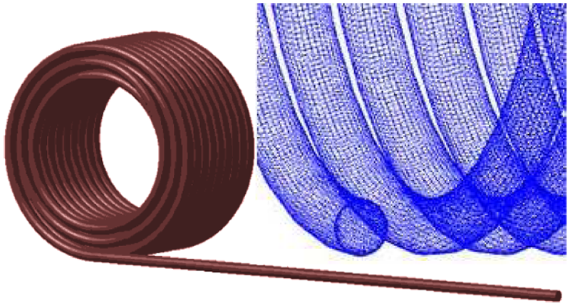
Three-dimensional rendering of the helical pipe and the whole computational grid.

A structured hexahedral multi-block grid was created with the grid generation tool ICEM CFD to mesh the entire computational domain, as shown in Figure 2. The mesh quality parameters like the determinant (larger than 0.65) and angle (larger than 36) indicate a perfectly regular mesh element. The grid independence was proven by comparing the simulation results (the unit pressure loss ΔP₀) with different numbers of grid elements from the coarsest to the finest, and the results are shown in Figure 3. With 75-mm pipe at 10 m³/h, for example, the unit pressure loss experiences a slight change (less than 2%) when the grid number is over 4.51 million, and it is more closer to the measured value when the grid number is 6.63 million, so the whole computational domain consists of 6.63 million grid elements. The y+ (non-dimensional distance from wall) value is at an order of magnitude of 1, which is suitable for automatic near-wall treatment in boundary layer.

Figure 2.

Details of the computational grid.

Figure 3.

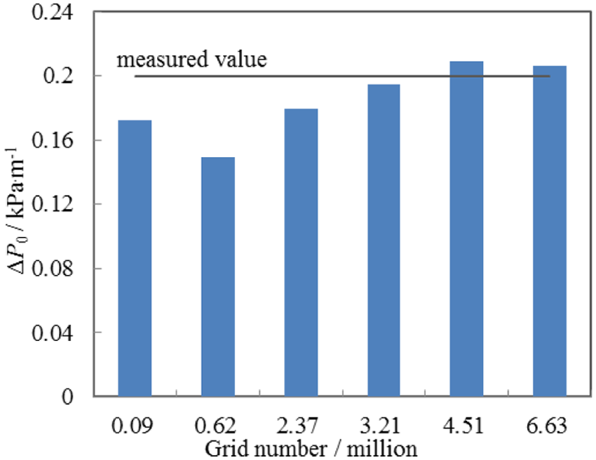
Grid-independence analysis.

Governing equations

The ANSYS-CFX code was used to solve the three-dimensional Navier–Stokes equations governing incompressible flow in several kinds of helically coiled pipes. The continuity and momentum equations can be written as

\frac{\partial}{\partial x_{i}} (ρ u_{i}) = 0

(1)

\frac{\partial}{\partial x_{j}} (ρ u_{i} u_{j}) = - \frac{\partial p}{\partial x_{i}} + \frac{\partial}{\partial x_{j}} [μ (\frac{\partial u_{i}}{\partial x_{j}} + \frac{\partial u_{j}}{\partial x_{i}})] + \frac{\partial}{\partial x_{j}} (- ρ \bar{u_{i}^{'} u_{j}^{'}})

(2)

where ρ is the density, µ is the dynamic viscosity, and $- ρ \bar{{u'}_{i} {u'}_{j}}$ is the Reynolds stress.

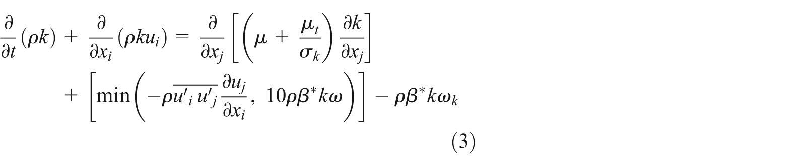
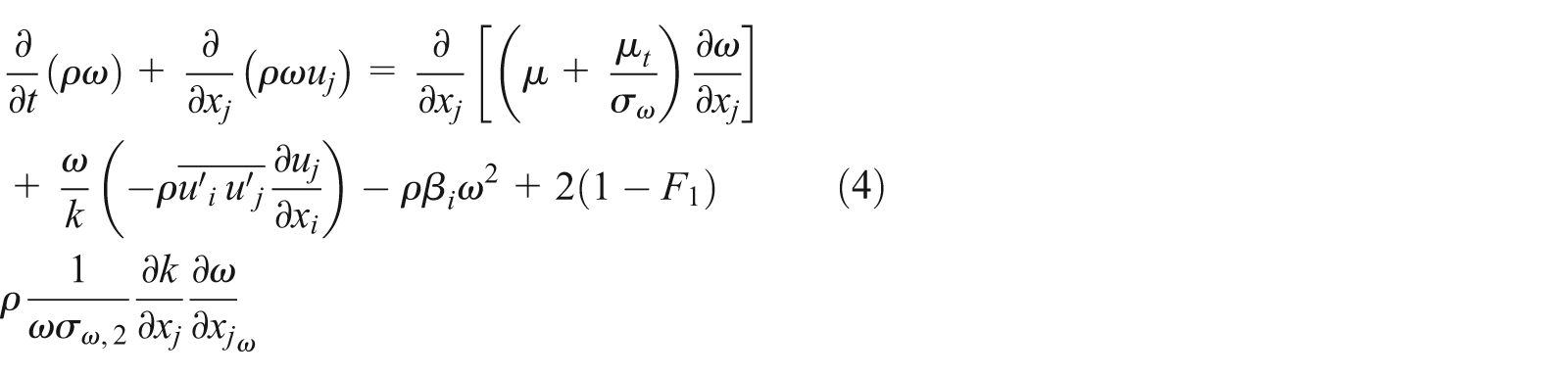
The turbulent pipe flow was simulated by the shear stress transport (SST) k − ω turbulence model. The turbulence kinetic energy k and the specific dissipation rate ω were obtained from the following transport equations

\frac{\partial}{\partial t} (ρ k) + \frac{\partial}{\partial x_{i}} (ρ k u_{i}) = \frac{\partial}{\partial x_{j}} [(μ + \frac{μ_{t}}{σ_{k}}) \frac{\partial k}{\partial x_{j}}] + [\min (- ρ \bar{{u^{'}}_{i} {u^{'}}_{j}} \frac{\partial u_{j}}{\partial x_{i}}, 10 ρ β^{*} k ω)] - ρ β^{*} k ω_{k}

(3)

\frac{\partial}{\partial t} (ρ ω) + \frac{\partial}{\partial x_{j}} (ρ ω u_{j}) = \frac{\partial}{\partial x_{j}} [(μ + \frac{μ_{t}}{σ_{ω}}) \frac{\partial ω}{\partial x_{j}}] + \frac{ω}{k} (- ρ \bar{{u^{'}}_{i} {u^{'}}_{j}} \frac{\partial u_{j}}{\partial x_{i}}) - ρ β_{i} ω^{2} + 2 (1 - F_{1}) ρ \frac{1}{ω σ_{ω, 2}} \frac{\partial k}{\partial x_{j}} {\frac{\partial ω}{\partial x_{j}}}_{ω}

(4)

where the turbulent viscosity µ_t is computed as follows

μ_{t} = \frac{ρ k}{ω} \frac{1}{max (\frac{1}{α^{*}}, \frac{S F_{2}}{α_{1} ω})}

(5)

where S is the strain rate magnitude and

β_{i} = F_{1} β_{i, 1} + (1 - F_{1}) β_{i, 2}

(6)

In these equations, the bending functions, F₁ and F₂, are given by

F_{1} = \tanh {{min [max (\frac{\sqrt{k}}{0.09 ω y}, \frac{500 μ}{ρ y^{2} ω}), \frac{4 ρ k}{σ_{ω, 2} max (2 ρ \frac{1}{σ_{ω, 2}} \frac{1}{ω} \frac{\partial k}{\partial x_{j}} \frac{\partial ω}{\partial x_{j}}, 10^{- 10}) y^{2}}]}^{4}}

(7)

F_{2} = \tanh {{[max (2 \frac{\sqrt{k}}{0.09 ω y}, \frac{500 μ}{ρ y^{2} ω})]}^{2}}

(8)

The following values are assigned to the model constants of the turbulence model: α^* = 1, α₁ = 0.31, β^* = 0.09, σ_k,₁ = 1.176, σ_k,₂ = 1.0, σ_ω,₁ = 2.0, σ_ω,₂ = 1.168, β_i,₁ = 0.075, and β_i,₂ = 0.0828.

Boundary conditions

At the inlet boundary, a uniform axial inlet velocity was prescribed together with a uniform turbulence intensity of 5%, whereas at the pipe outlet, the relative static pressure was fixed to zero. A no-slip condition was imposed on the wall. The governing equations were solved in a stationary framework. The high resolution was used in advection scheme and turbulence numeric, and the convergence criterion was set as 10⁻⁵.

Results and discussions

Experimental validation

Experimental data for the water sprayer were collected to verify the accuracy of the calculation. A schematic representation of the test system is shown in Figure 4. Two pressure gauges were mounted at the inlet of the water sprayer and before the entrance of the sprinkle nozzle to measure the pressure loss of the helical pipe. The pressure gauge is a mechanical spring type with a pointer and it has an estimated experimental uncertainty of 0.4%. An electromagnetic flowmeter is used with an estimated experimental uncertainty of 0.5%. The working fluid is water, which was drawn from a well using a submerged pump.

Figure 4.

Sketch of the test rig: (1) submerged pump, (2) valve, (3) flowmeter, (4) water sprayer, and (5) pressure gauge.

The measurements and numerical results are presented in terms of the unit pressure loss ΔP₀ = (P_in − P_out) / L, where P_in is the pipe-inlet pressure, P_out is the pipe-outlet pressure, and L is the length of the pipe. The comparison of pressure losses obtained by both numerical calculations and experiments for all kinds of pipes are shown in Figure 5. Each experimental point is the average among several equivalent measurements with an error bar representing one standard deviation of uncertainty. From Table 1, it can be seen that the results of both methods have an acceptable agreement, and the mean relative errors are all less than 5%, which validates the CFD model over the present range of flow conditions.

Figure 5.

Comparisons of numerical calculation and experimental data.

Table 1.

Accuracy of numerical calculation.

	50 mm	65 mm	75 mm	90 mm
Average absolute difference (kPa)	0.64	0.09	0.07	0.02
Maximum relative error (%)	9.6	7.6	8.94	8.29
Mean relative error (%)	4.82	3.46	4.05	3.92

Flow characteristics under various coil diameters

The bending extent of the helically coiled pipe will give rise to various patterns of secondary vortex, the flow fields will change with different secondary flow patterns. The different bending extents can be represented as the various reel diameters and coiling layers for the water sprayer. Figure 6(a) shows the unit pressure loss for different coil diameters ranging from 300 to 3000 mm with the pipe diameter of 75 mm. The unit pressure loss rises with increasing flow discharge, and reduces with increasing coil diameter at a given flow rate. Figure 6(b) shows that the unit pressure loss experiences a drastic decline and then a negligible gentle decline with the increase in the coil diameter under the fixed flow discharge of 10 m³/h. The unit pressure drop rate has the significant shift around 1300 mm in coil diameter. This phenomenon implies that increasing the coil diameter is an effective method for reducing the pressure loss when the coil diameter is less than 1300 mm, otherwise it is unsuccessful.

Figure 6.

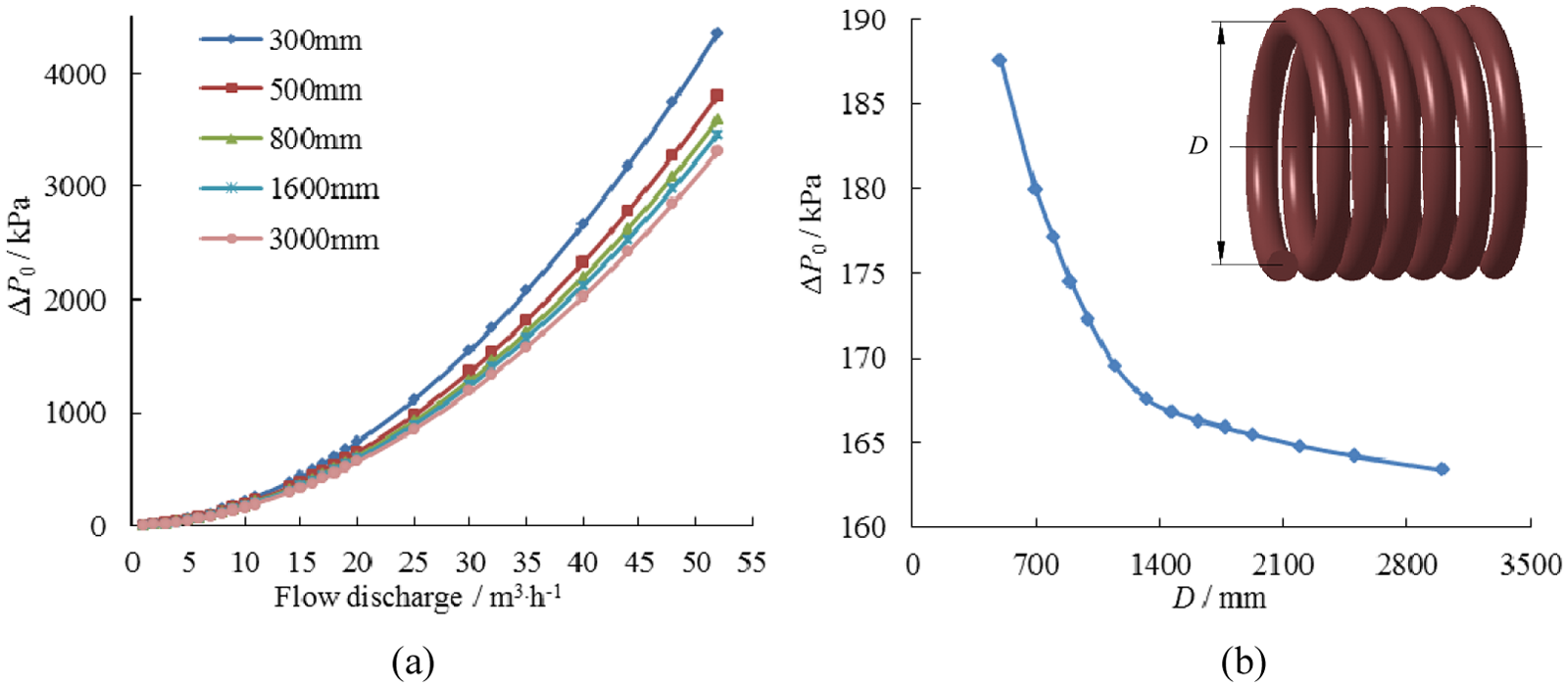
Unit pressure losses for different coil diameters: (a) variation of unit pressure loss with flow discharge and (b) variation of unit pressure loss with coil diameter under fixed flow discharge.

The secondary vortex pattern was described by the streamline in cross section which was perpendicular to the major flow. The flow contains a pair of counter-rotating vortices, and the double secondary vortices turn and deform with the variation of coil diameter, as shown in Figure 7. The line of vortex centers was used to locate the secondary vortices, and the angle between the line of centers and the horizontal diameter was used to quantify the extent of change of the secondary vortices’ location, and the observed cross section was selected at the half length of the coiled pipe. The location of the secondary vortex is 67° at the coil diameter of 300 mm, and then totally turns 45° in clockwise direction to 22° at the coil diameter of 3000 mm; it decreases with the increasing coil diameter. The streamline is distorted when the coil diameter is less than 1300 mm, and then it becomes smooth when the coil diameter exceeds 1300 mm. Therefore, the variation of secondary vortices can be attached to the change of the unit pressure loss since the significant changes both start from the coil diameter of 3000 mm, and then it can be obtained that the overlarge deflection angle and the distorted streamline will generate the higher unit pressure loss under the same pipe diameter. As shown in Figure 7(a)–(c), the deflection angles of the secondary vortices are larger than 45°, the distorted streamline diffuses the vortices and makes the line of vortices centers off the cross section center. These performances result in an unstable flow field, and the unit pressure loss falls sharply with the rise in the coil diameter. Then, from Figure 7(d)–(f), the deflection angle goes down to smaller than 45°, the streamline becomes smooth, and the secondary vortices mode varies from diffusion to intensification. Hence, the flow field begins to stabilize, and the unit pressure loss has no substantial change with the increase in coil diameter.

Figure 7.

Vortices locations for different coiling diameters: (a) D = 300 mm, (b) D = 500 mm, (c) D = 800 mm, (d) D = 1300 mm, (e) D = 1900 mm, and (f) D = 3000 mm.

The mode of the secondary vortices will lead to various radial velocity fields. The magnitude of the radial velocity gradually decreases with the increase in the coil diameter, as shown in Figure 8. The high radial velocity tends to increase in the intensification and distortion regions of the streamline, whereas the low velocity tends to increase in the central regions of the double vortices. The intensification regions appear on the right and left sides of the cross section (both vortices borders), and the distortion regions appear on the left lower side of the cross section (inner side of the bottom vortex) when the coil diameter is less than 1300 mm.

Figure 8.

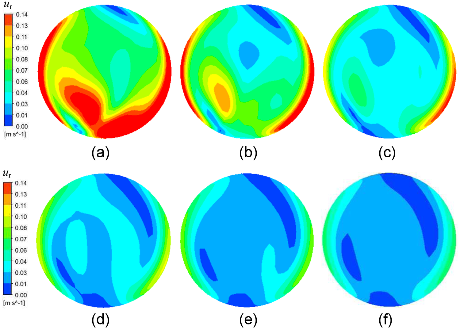
Radial velocity field for different coiling diameters: (a) D = 300 mm, (b) D = 500 mm, (c) D = 800 mm, (d) D = 1300 mm, (e) D = 1900 mm, and (f) D = 3000 mm.

To analyze the pipe flow in detail, the median horizontal line and vertical line were extracted from the cross section. The distance away from the left wall in horizontal line was defined as x, and the distance away from the inner wall in vertical line was defined as y. The upside of the cross section was defined as the outer wall, and the downside was defined as the inner wall, that is, the coiling axial of the helically coiled pipe is on the downside, as shown in Figure 9.

Figure 9.

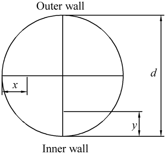
Cross-section normal to the primary flow direction.

The distribution of turbulence dissipation rate (ε) in the cross section is described by the two lines, as shown in Figure 10. The profiles of both lines present a slight fluctuation with an increase in coil diameter and then remain stable until the coil diameter increases to 1300 mm, while the value in the central region is always lower than the value near the wall. The profile of the turbulence dissipation rate on horizontal line shows a symmetrical curve with the same lower value in the central region under stable state. The profile on vertical line displays a reducing trend from the inner wall side to the outer wall side in the central region under stable state.

Figure 10.

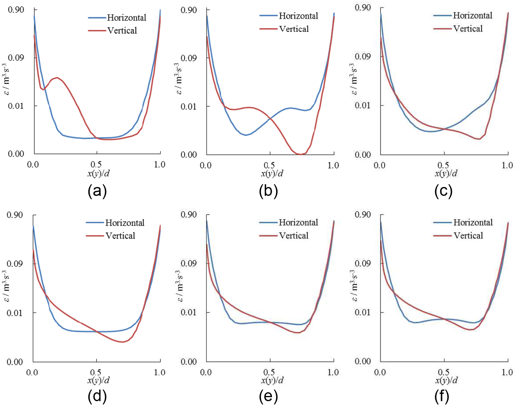
Distribution of turbulence dissipation rate on horizontal and vertical lines for different coiling radii: (a) D = 300 mm, (b) D = 500 mm, (c) D = 800 mm, (d) D = 1300 mm, (e) D = 1900 mm, and (f) D = 3000 mm.

The secondary vortex intensity $(J_{ABS}^{n})$ can also illustrate the flow filed in the helically coiled pipe. It is a main factor for the secondary flow characteristics. It can be described by the absolute vorticity flux in normal direction of cross section²⁶

J_{ABS}^{n} = \frac{1}{A} \int \int_{A} | ω^{n} | dA

where A is the area of cross section (m²), n represents the normal direction of the cross section, and ω is the vorticity. The vorticity is defined as the curl of the flow velocity u, and the definition can be expressed as follows

ω = \nabla \times u

The absolute vorticity flux in normal direction transforms from the patchy distribution to the vertically symmetrical distribution, and the value decreases with the increase in coil diameter, as shown in Figure 11. The higher values all appear on the right and left sides of the cross section, which are similar to the radial velocity distribution, for both of them are generated by the secondary flow. The distribution in central area is irregular when the coil diameter is less than 1300 mm. However, it closes on a consensus when the diameter exceeds 1300 mm.

Figure 11.

Contours of secondary vortex intensity for different coiling diameters: (a) D = 300 mm, (b) D = 500 mm, (c) D = 800 mm, (d) D = 1300 mm, (e) D = 1900 mm, and (f) D = 3000 mm.

Figure 12 displays the change curve of the secondary flow intensity with the pipe diameter of 75 mm, it has the same variation trend to the unit pressure loss. The secondary flow intensity experiences a rapid fall, followed by a slow decline, and the turning point is around 1300 mm in diameter. Hence, the secondary vortex is the major component contributing to the variation of unit pressure loss.

Figure 12.

Variation of secondary flow intensity with coiling radius pipe diameters.

Flow characteristics under different pipe diameters

Several commonly used pipe diameters with a given coil diameter (D = 800 mm) were selected to analyze the effect of four different pipe diameters on the flow field. Figure 13 shows that the unit pressure loss increases with flow discharge for a given pipe diameter but decreases for a given flow rate with the increase in pipe diameter. It can also be seen that the growth rate of the unit pressure loss for a 50-mm-diameter pipe is higher than the other pipes obviously, especially when the flow discharge increases above 10 m³/h, the growth rate rises sharply. It means that a 50-mm pipe is inappropriate when the flow discharge exceeds 10 m³/h.

Figure 13.

Pressure losses for different pipe diameters.

Figure 14 presents the variation of vortices’ locations for different pipe diameters with the same flow discharge (10 m³/h) and the same coil diameter. The vortex-deflection angle rises with the increase in pipe diameter, and the streamlines change from a smooth to a distorted pattern. According to the above analysis, for a given pipe diameter, the vortex-deflection angle will increase with the increase in coil diameter; meanwhile, the streamline will develop from a distorted to a smooth pattern, and the unit pressure loss will be higher in the condition of a larger vortex-deflection angle or a distorted streamline. Therefore, the flow in 50-mm pipe has developed to the stabilization state with smooth streamline, and the unit pressure loss has no drastic alternation with the following increase in coil diameter. However, the other pipes have not developed to the stabilization states, and their unit pressure losses have not attained to the optimum. The flow characteristics such as the turbulence dissipation rate, the vorticity, and the secondary flow intensity for different pipe diameters are shown in Figures 15 and 16. Their distributed forms are similar, only have the differences in magnitude. The value of each characteristic reduces with the increase in pipe diameter, and the decline rate from 50 to 60 mm in diameter is the highest. The profiles of turbulence dissipation rate in horizontal line are all like U-shaped curves, and in vertical line, all are like V-shaped curves and the minimum values biased toward the outer wall side. The contours of the secondary flow intensity display almost vertical symmetric distribution with the relatively higher value near left and right walls.

Figure 14.

Vortices’ locations for different pipe diameters: (a) 50 mm, (b) 65 mm, (c) 75 mm, and (d) 90 mm.

Figure 15.

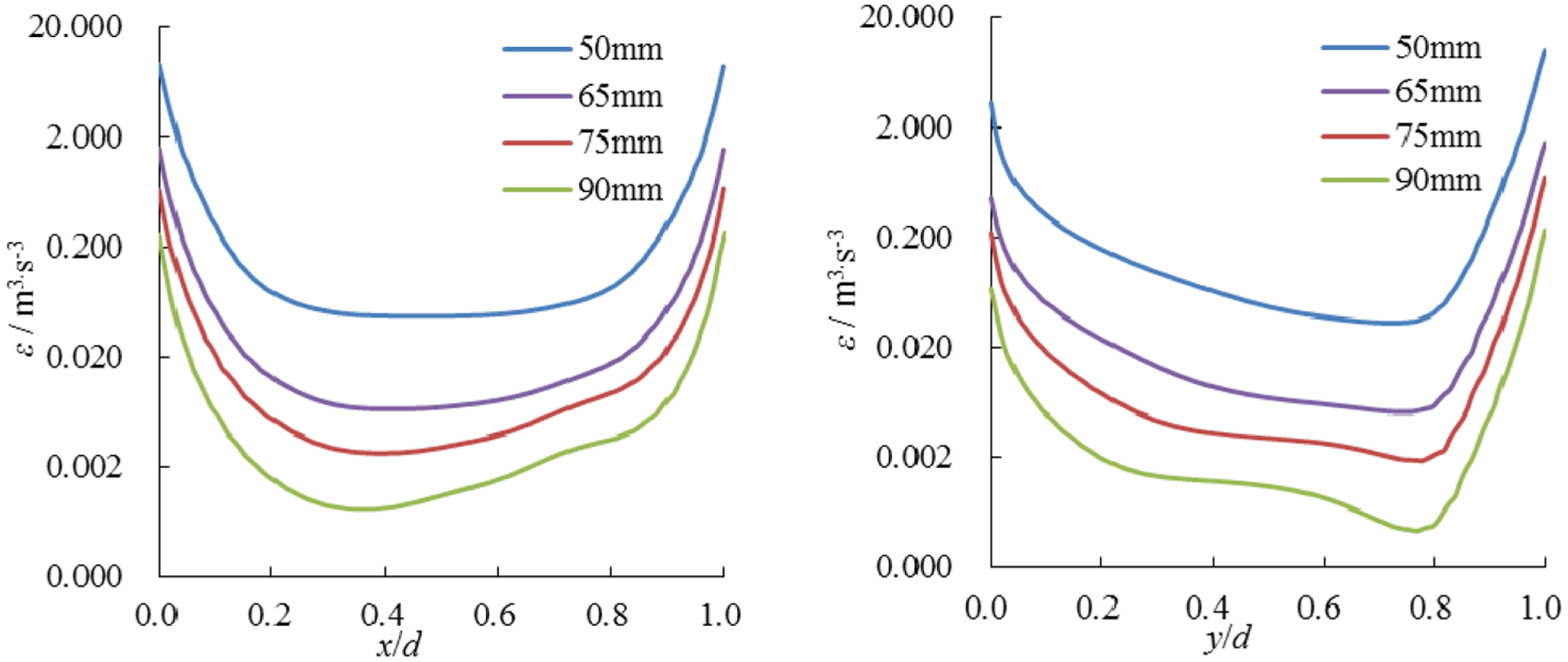
Distributions of turbulence dissipation rate for different pipe diameters.

Figure 16.

Contours of secondary flow intensity for different pipe diameters: (a) 50 mm, (b) 65 mm, (c) 75 mm, and (d) 90 mm.

Conclusion

CFD predictions of the pressure losses and secondary flow characteristics in the helically coiled pipe were presented. The CFD methodology was validated by comparing the numerical results with experimental data. The mean deviation between the measured and simulated pressure losses was less than 5%.

The pressure loss is affected by the pipe geometry. The pipe flow becomes stable with the increase in coil diameter for the definite pipe diameter, and in the meantime, the unit pressure experiences a gradual reduction with different droop rates. In addition, the development of pipe flow slows down with the increase in pipe diameter due to the enlarged flow area, so the coil diameter of beginning stable state has an enhancement.

The unit pressure loss has close relation with the secondary flow pattern for a given pipe diameter. Both the larger vortex-deflection angle and the distorted streamline will enhance the unit pressure loss. The unit pressure loss experiences a significant reduction with the decline in vortex-deflection angle until 45°, and in the meantime, the extent of streamline distortion gradually decreases. Then, the unit pressure loss has no obvious shift when the deflection angle is less than 45°, and the pipe flow develops to the stabilized state with the smooth streamline in cross section simultaneously.

The flow characteristics such as the turbulence dissipation rate and the secondary vortex intensity vary with the development of the pipe flow. Their values decline until the pipe flow reaches the steady state. Their contours change from the random distribution to regular and symmetrical distribution.

This study can provide suggestions in improving the performance of water sprayers.

Footnotes

Academic Editor: Roslinda Nazar

Declaration of conflicting interests

The author(s) declared no potential conflicts of interest with respect to the research, authorship, and/or publication of this article.

Funding

The author(s) disclosed receipt of the following financial support for the research, authorship, and/or publication of this article: This research was supported by the National Key Research Programs (no. 2016YFC0400104) and the National Studying Abroad Foundation of China and Graduate Student Innovation Projects of Jiangsu Province (grant no. CXLX13_660).

References

Ghobadi

Muzychka

. Pressure drop in mini-scale coiled tubing. Exp Therm Fluid Sci 2014; 57: 57–64.

Liu

Afacan

Nasr-El-Din

. An experimental study of pressure drop in helical pipes. P Roy Soc A: Math Phy 1994; 444: 307–316.

Kim

Son

. An experimental study on the pressure drop and heat transfer through straight and curved small diameter tubes. J Mech Sci Tech 2014; 28: 797–809.

Salem

Elshazly

Sakr

. Effect of coil torsion on heat transfer and pressure drop characteristics of shell and coil heat exchanger. J Therm Sci Eng Appl 2016; 8: 011015–1–7.

Manlapaz

Churchill

. Fully developed laminar flow in a helically coiled tube of finite pitch. Chem Eng Commun 1980; 7: 57–78.

Gupta

Wanchoo

Jafar Ali

TRM

. Laminar flow in helical coils: a parameter study. Ind Eng Chem Res 2011; 50: 1150–1157.

Ali

. Pressure drop correlations for flow through regular helical coils. Fluid Dyn Res 2001; 12: 295–301.

Wang

. On the low-Reynolds-number flow in a helical pipe. J Fluid Mech 1981; 108: 185–194.

Germano

. On the effect of torsion on a helical pipe flow. J Fluid Mech 1982; 125: 1–8.

10.

Germano

. The Dean equations extended to a helical pipe flow. J Fluid Mech 1988; 203: 289–305.

11.

Austin

Seader

. Fully developed viscous flow in coiled circular pipes. AIChE J 1973; 19: 85–94.

12.

Kao

. Torsion effect on fully developed flow in a helical pipe. J Fluid Mech 1987; 184: 335–356.

13.

Xie

. Torsion effect on secondary flow in a helical pipe. Int J Heat Fluid Flow 1990; 11: 114–119.

14.

Chen

Jan

. The characteristics of laminar flow in a helical circular pipe. J Fluid Mech 1992; 244: 241–256.

15.

Vasudevaiah

Patturaj

. Effect of torsion in a helical pipe flow. Int J Math Math Sci 1994; 17: 553–560.

16.

Zhang

. Fluid flow in a helical pipe. Acta Mech Sinica 1999; 15: 299–312.

17.

Boersma

Nieuwstadt

FTM

. Large-eddy simulation of turbulent flow in a curved pipe. J Fluid Eng: T ASME 1996; 118: 248–254.

18.

Yamamoto

Yanase

Yoshida

. Torsion effect on the flow in a helical pipe. Fluid Dyn Res 1994; 14: 259–273.

19.

Yamamoto

Akita

Ikeuchi

. Experimental study of the flow in a helical circular tube. Fluid Dyn Res 1995; 16: 237–249.

20.

Yamamoto

Yanase

Jiang

. Stability of the flow in a helical tube. Fluid Dyn Res 1998; 22: 153–170.

21.

Noorani

Khoury

GKE

Schlatter

. Evolution of turbulence characteristics from straight to curved pipes. Int J Heat Fluid Flow 2013; 41: 16–26.

22.

Jayakumar

Mahajani

Mandal

. CFD analysis of single-phase flows inside helically coiled tubes. Comput Chem Eng 2010; 34: 430–446.

23.

Hüttl

Friedrich

. Influence of curvature and torsion on turbulent flow in helically coiled pipes. Int J Heat Fluid Flow 2000; 21: 345–353.

24.

Hüttl

Friedrich

. Direct numerical simulation of turbulent flows in curved and helically coiled pipes. Comput Fluids 2001; 30: 591–605.

25.

Hayamizu

Yamamoto

Yanase

. Experimental study of the flow in helical circular pipes: torsion effect on the flow velocity and turbulence. J Therm Sci 2008; 17: 193–198.

26.

Lin

Sun

Wang

. The relationship between absolute vorticity flux along the main flow and convection heat transfer in a tube inserting a twisted tape. Heat Mass Transfer 2009; 45: 1351–1363.

Secondary vortex-based analysis of flow characteristics and pressure drop in helically coiled pipe

Abstract

Keywords

Introduction

Materials and methods

Geometry and calculation grids

Governing equations

Boundary conditions

Results and discussions

Experimental validation

Flow characteristics under various coil diameters

Flow characteristics under different pipe diameters

Conclusion

Footnotes

Declaration of conflicting interests

Funding

References