A simple method for high-precision evaluation of valve flow coefficient by computational fluid dynamics simulation

Abstract

Flow coefficient is an important performance index associated with the energy efficiency of a valve, and an effective method to evaluate valve flow coefficient is necessary for valve industry. However, theoretical estimation often results in poor accuracy, while experimental measurements involve significant costs in time and equipment. In this article, a computational fluid dynamics method is proposed to achieve simple and accurate evaluation of valve flow coefficient. For each valve, a computational fluid dynamics model is established containing a valve section, an upstream section, and a downstream section. A grid-adaptation strategy is then applied to improve the accuracy of simulation. To calculate flow coefficient, the most important issue is to determine the net pressure loss induced by valve (ΔP_v). Herein, the overall pressure drop (ΔP_o) is obtained first, and the pipe-induced pressure drop (ΔP_p) is estimated by linear fitting. Then, ΔP_v is calculated as the difference between ΔP_o and ΔP_p. To ensure accurate estimation of the pressure losses, a length of 26 times of pipe diameter is preferred for the upstream section. The experiments demonstrated that the presented method can accurately predict flow coefficient for various types of valves and thus has great potential to be widely used in the valve industry.

Introduction

Valves are widely used in many industry environments, and their performances have direct impact on the stability and efficiency of the entire system. To describe the performance of a valve, flow coefficient is commonly used, and higher valve of flow coefficient often means better energy efficiency. When the valve industry pays more and more effort on improving the flow efficient of valves to fulfill the new energy conversation requirement, a convenient and accurate method to evaluate valve flow coefficient becomes unprecedentedly important.

Currently, the evaluation of valve flow coefficient is often performed by theoretical estimation or experimental measurement. Theoretical estimation cannot reflect the influence of detailed valve structure, and thus often results in poor accuracy.^1,2 Experimental measurement requires significant costs in time and equipment.^2,3 Especially for some valves that involve extraordinary dimension or structure, it is difficult to measure their flow coefficients experimentally.^4–6 Furthermore, experimental method can only provide limited data at several preset locations, and the interaction between valve structure and flow characteristics is still unrevealed,^4,7,8 so it is difficult to optimize a valve design according to experimental results.

With the recent development of computational fluid dynamics (CFD), it is possible to simulate and visualize a complex flow field and then help designers learn about more interesting details of flow field. Therefore, CFD simulation can be an effective alternative to experimental method to evaluate the performance of valves, and a lot of attempts had been made with the help of different software.^2–12 For example, Huang and Kim ¹⁰ investigated the flow characteristics of a butterfly valve at different valve disk angles with a uniform incoming velocity using FLUENT. Vescovo and Lippolis ⁹ also used FLUENT to analyze the flow forces acting on spools of hydraulic directional control valves and compared the accuracies resulted from two-dimensional (2D) and three-dimensional (3D) models. Leutwyler and Dalton ³ studied the flow field, resultant force, and aerodynamic torque on a butterfly valve in a compressible fluid using CFX. Song and Park ¹¹ evaluated the flow coefficient and hydrodynamic torque coefficient of a large butterfly valve at various opening degrees using CFX. Aung et al. ⁵ compared the flow forces and energy loss characteristics in a flapper–nozzle pilot with different null clearances.

CFD simulation was also used to investigate the dynamic characteristics of valves.^4,6,13,14 For example, Srikanth and Bhasker ¹⁴ investigated the compressible air flow in the valve of a puffer chamber using moving grid technique in CFD simulation. Qian et al. ¹³ studied the opening process of a pilot-control globe valve through a user-defined function (UDF) program of the valve core’s movement. Song et al. ⁴ investigated the dynamic characteristics of a safety relieve valve using CFX. Saha et al. ⁶ investigated the dynamic simulation of a pressure-regulating valve using FLUENT, providing a tool to predict the spool movement and the final spool position.

Furthermore, CFD simulation has shown great feasibility in adapting to different valve types and geometries and thus provides a useful tool for valve design and optimization.^15–19 Whitehead et al. ¹⁷ tried to improve the performance of a valve by changing various aspects of the internal flow path. Song et al. ¹⁶ proposed a multidisciplinary optimization of a butterfly valve with the help of CFD simulation. Lisowski and Rajda ¹⁵ designed a new directional control valve with the help of CFD analysis. Ye et al. ¹⁸ investigated the influence of different spool groove shapes on the valve flow characteristics using both CFD and experimental investigations, and the results agreed well with each other.

Although previous studies have well demonstrated that CFD simulation can be a useful tool for valve analysis and optimization, the detailed CFD method for evaluation of valve flow coefficient has not been seriously discussed. In fact, some of the details, such as the modeling and meshing strategies, have great impact on evaluation accuracy and efficiency. For example, if the upstream section in a CFD model is not long enough, the simulated flow may not be fully developed before entering the valve section, violating the essential requirement for flow coefficient calculation. Unfortunately, the CFD models in the current methods seem to be established empirically without serious examination, thus likely to cause significant error. Meshing is another important step influencing the accuracy of CFD simulation. In the current methods, this step often involves a lot of empirical refinement, which is very difficult and time consuming. Moreover, the over-reliance on individual experience of this process also induces some uncertainty in simulation accuracy. Those issues may partially be the reason why unfavorable results (relative errors more than 49%) occurred when evaluating flow coefficient by simulation in certain cases. ¹¹

To date, CFD simulation has not been widely used for evaluation of valve flow coefficient, especially in China where most of the valve designers lack advanced CFD experience. In this article, a new CFD simulation method is presented to achieve simple and accurate evaluation of valve flow coefficient. A uniform modeling strategy is proposed, and a semi-automatic mesh strategy is also applied. In this manner, the CFD method can be easily used in valve industry, and the consistency of calculation can be ensured among operators. Validation experiments show that the presented method can achieve high-accuracy evaluation of valve flow coefficients and thus provide effective tool for improving valve energy efficiency.

Principle of calculation

Depending on what unit system is used, flow coefficient can be given as K_v or C_v, both of which are defined as the flow rate though of a valve with a certain pressure drop across the valve. For example, C_v can be calculated as below^1,11,19,20

$$C_v=Q\times \sqrt{\frac{G}{\Delta P_v}}$$

(1)

where Q is the flow rate (gal/min), ΔP_v is the net pressure drop induced by the valve (lbf/in²), and G is the specific gravity of the working fluid. Alternatively, when Q is in units of cubic meter per hour and ΔP_v is in units of bar, K_v can be calculated. In industry, C_v can also be calculated as 1.156 times of K_v. ²⁰

The most difficult issue in calculating C_v/K_v is to determine the value of ΔP_v because it cannot be simply taken as the pressure difference across the valve. In a standard experimental protocol, P_v is calculated by subtracting the net pressure loss in the pipe (ΔP_p, obtained with a “pipe-only” flow) from the overall pressure drop (ΔP_o, obtained with a “pipe-valve” flow).^20,21 In CFD simulation, we can apply a similar strategy, that is, modeling a “valve-pipe” flow and a “pipe-only” flow separately to calculate ΔP_o and ΔP_p. However, this approach involves obvious waste in human labor and computing resource. Hence, a simpler and more efficient CFD method is required to calculate P_v.

According to Darcy–Weisbach formula, the pressure loss in a fully developed pipe flow can be given as ²¹

$$h_f=\lambda \frac{l}{D}\frac{V^2}{2g}$$

(2)

where λ is the friction loss factor which is related to surface roughness and Reynolds number, l is the pipe length (m), D is the inner diameter (m) of the pipe, V is the average flow rate (m/s), and g is the gravitational acceleration (m/s²). It is shown that the friction loss pressure varies linearly with the length of the pipeline under normal condition. Thus, it is proposed herein to predict ΔP_p by linear fit according to the pressure distribution in the upstream section.

CFD simulation

Modeling

In this study, each CFD model includes an upstream section, a valve section, and a downstream section, as shown in Figure 1. The length of the downstream section (L_d) was set to be 10 times of D according to the experimental method,^19,20 while the length of upstream section (L_u) was set as a variable in the range of 11D–41D. For each valve, those models with different L_u were simulated with the same parameter setting and operation procedure. The results were analyzed and compared to determine the optimum length of upstream section for the ease and accuracy of prediction of ΔP_p.

Figure 1.

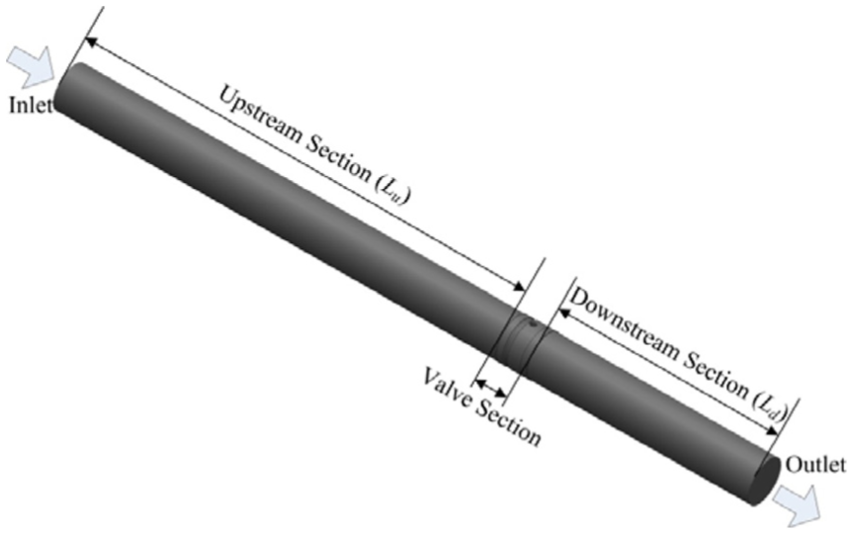
Illustration of the CFD model used for simulation and calculation.

Mesh generation and adaptation

To reduce the difficulty and workload, an automatic mesh strategy is used. For each model, an initial mesh was generated automatically by commercial software, ICEM CFD. Hexahedral mesh was used for both upstream section and downstream section, while tetrahedral mesh was used for valve section. Four different mesh sizes were compared, and the finally selected one has 2 million cells in total. To further improve the mesh quality, grid-adaptation techniques were applied subsequently.

Considering there are significant velocity and pressure gradients near the wall, Y plus grid-adaptation technique was first used to refine or coarsen grids in the boundary area. In addition, there are often drastic changes in flow velocity and pressure near the gap between the valve spool and the seat. Hence, velocity gradient grid adaptation is also used to refine grids near the valve spool. For Y plus grid adaptation, the minimum threshold and maximum threshold were set to be 30 and 200, respectively. For velocity gradient grid adaptation, the normalization option is standard, and the encryption threshold was determined by high-gradient area of adaptive function contour. For each model, the velocity gradient grid adaptation was used only once, while the Y plus grid adaptation was used continuously till the value of Y plus fell between 30 and 300. ²²

Simulation setting

In this study, the boundary conditions are specified as mass flow rate inlet, pressure outlet, and non-slipping wall. The fluid medium was set as water with a viscosity of 0.001003 kg/m s and a density of 998.2 kg/m³, respectively. The type of flow can be determined on the basis of the calculated value of the Reynolds number. Standard k–ε equations shown below were chosen to model the turbulent flow, since previous studies have demonstrated that this model can provide favorable accuracy for simulation of complex flow in valves^4,5,12–14

$$\frac{\partial }{\partial t}(\rho \kappa )+\nabla ·(\rho \kappa \stackrel{\rightharpoonup }{u})=\nabla ·[(\mu +\frac{{\mu }_t}{{\sigma }_{\kappa }})\nabla \kappa ]+G_{\kappa }-\rho \epsilon$$

(3)

$$\frac{\partial }{\partial t}(\rho \epsilon )+\nabla \cdot (\rho \epsilon \stackrel{\rightharpoonup }{u})=\nabla \cdot \left[\left(\mu +\frac{{\mu }_t}{{\sigma }_{\epsilon }}\right)\nabla \epsilon \right]+\frac{\epsilon }{\kappa }(C_{1\epsilon }{G}_{\kappa }-C_{2\epsilon }\rho \epsilon )$$

(4)

where the turbulent viscosity, µ, is computed by combining k and ε as follows

$$\mu =C_{\mu }\rho \frac{{\kappa }^2}{\epsilon }$$

(5)

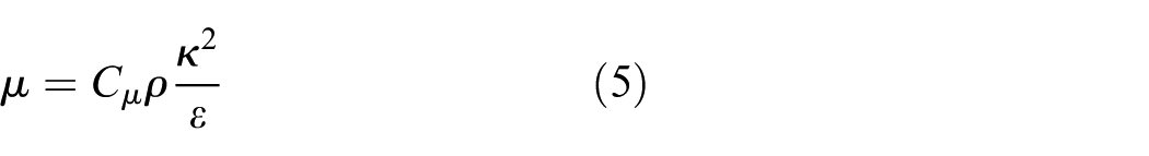
In the above equations, C_1ε, C_2ε, C_3ε, and C_µ are the empirical constants and G is the turbulence production term. This standard model is used without any further modifications, and default values were used for the constants. In addition, standard wall functions were adopted for near-wall treatment. During simulation, second-order upwind scheme was used and SIMPLE algorithm was chosen to resolve the governing equations since it is more memory-efficient than the latter and better adapts to the computationally expensive grids. Iterative convergence was at least three (preferably four) orders of magnitude decrease in the normalized residuals for each equation solved.

Data processing

After convergence, ΔP_o can be obtained easily as the pressure difference between the inlet and the outlet for each model, while ΔP_p needs further estimation by curve fitting according to the pressure distribution in the upstream section.

For each modeled upstream section, the averaged pressure values on different cross sections can be extracted, and an axial pressure distribution curve can be plotted. Linear fitting was then performed to predict another “whole length pressure drop” corresponding to a dummy pipe-only situation. In this manner, ΔP_p was estimated, and then ΔP_v can be obtained. Finally, the valve flow coefficient can be calculated according to equation (1).

To evaluate the accuracy of the linear fitting estimation of ΔP_p, additional “pipe-only” models were also established and simulated. The deviation between the estimated value by a “pipe-valve” model and the directly calculated value by the corresponding “pipe-only” model was considered as the error of such linear fitting estimation.

Experimental validation

To validate the accuracy of CFD method, a series of experiments were also conducted. The experimental system was established according to the industry standard,^20,21 as shown in Figure 2. Various types of valves, including butterfly valves, camflex valves, and sleeve valves, were tested for comparison with simulation. The operation procedures were also conducted following the standard method. For each valve, 10 times of tests were performed, and the averaged value was finally used.

Figure 2.

The experimental system: (a) the laboratory and (b) sketch of the system. (1) Water supply, (2) flow meter, (3) thermometer, (4) and (9) regulating valves, (5) and (8) pressure tapping points, (6) upstream pressure measuring device, (7) valve under test, and (10) differential pressure measuring device.

Results and discussion

For each model, several rounds of pilot simulation were performed first to improve the mesh quality. Generally, the mesh quality can be effectively improved after a round of gradient adaptation and one to two rounds of Y plus adaptation, as shown in Figure 3.

Figure 3.

Illustration of the mesh adaptation: (a) mesh grid near the valve before adaptation, (b) mesh grid near the valve after adaptation, (c) mesh grid near the wall before adaptation, and (d) mesh grid near the wall after adaptation.

With the adapted mesh model, a final round of simulation was performed. After convergence, the field variables such as velocity vectors, velocity magnitude, and pressure are available for all grid points in the computational domain for visualization and interpretation through contour plots, velocity vectors, and streamlines. A set of typical contour plots with respect to a DN500 butterfly valve flow (D = 500 mm, L_u = 21D, L_d = 10D, Q = 1624.60 m³/h) is shown in Figure 4 as an example. It is clearly indicated that the valve causes interference to the flow distribution not only in the valve section but also in the upstream and downstream sections. That is why ΔP_v should not be simply calculated as the pressure difference across the valve section. To avoid this problem, we proposed to calculate ΔP_v by subtracting the net pressure loss induced by pipe (ΔP_p) from the overall pressure loss (ΔP_o) in a “pipe-valve” flow.

Figure 4.

Contours of (a) pressure and (b) velocity near the spool of a DN500 butterfly valve spool.

For the DN500 butterfly valve flow illustrated above, ΔP_o can be easily calculated as 4.2836 kPa based on the simulated result. To estimate ΔP_p, the axial pressure distribution in the upstream section was plotted as shown in Figure 5(a). The curve can be divided into three segments, corresponding to the developing flow near the inlet, the developed flow in the middle, and the valve-interfered flow near the valve, respectively. To achieve accurate estimation of ΔP_p, the values on six sequential cross sections in the middle part were used for curving fitting. The fitted formula was y = 0.0306x + 0.0936, by which ΔP_p can be calculated as 1.0422 kPa given x = 31 (because the total pipe length was equal to L_u + L_d = 31D). Correspondingly, ΔP_v can be calculated as ΔP_v = ΔP_o − ΔP_p = 3241.4 Pa and then K_v = 9023.0728.

Figure 5.

Simulated (a) pressure distribution and (b) pressure drops in the upstream section of a DN500 butterfly valve flow, in which the total length of the upstream section is 21 times of pipe diameter (D).

It is clear that the calculated result is highly depended on the estimation of ΔP_p. To evaluate the accuracy of such linear fitting method, an additional “pipe-only” model (D = 500 mm, L = 31D) was established and simulated for comparison. The resulted ΔP_p was 1028.43 Pa, according to which the relative error of the estimation was only 1.34%, indicating a very good accuracy. Further investigation indicated that this estimation accuracy can be further improved by extending the upstream section in the CFD model. However, if the upstream section is too long, much more computing resource should be cost. It is necessary to determine an optimum L_u to balance the requirements in both accuracy and efficiency. This work was performed herein by comparing the estimated errors resulted from a series of models with different lengths of L_u for the same valves.

Figure 6 illustrates the evaluated errors corresponding to the CFD models with different L_u. For the DN500 butterfly valve, it is shown that the curves tend to converge when the upstream section is longer than 26D regardless of the inlet flow rate. Similar results were also observed for another DN100 diaphragm valve. Therefore, it is feasible to regard 26D as an optimum length for modeling the upstream section of a valve flow.

Figure 6.

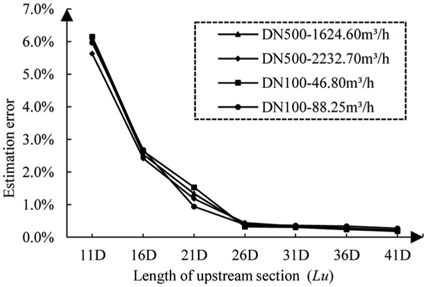
Relative error of linear fitting estimation of ΔP_p.

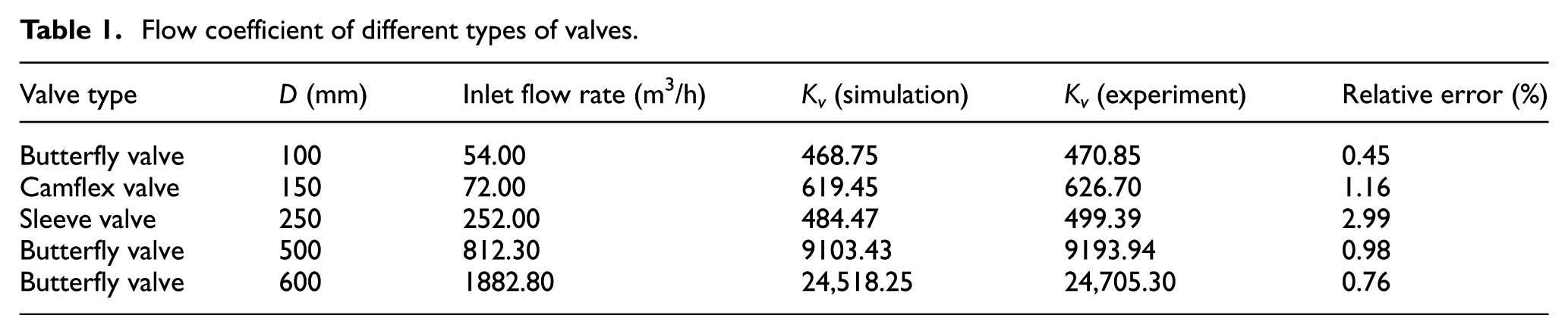
In order to further validate the proposed approach, a series of simulations and experiments were performed on different types of valves, including a DN100 concentric butterfly valve, a DN150 camflex valve, a DN250 sleeve valve, a DN500, and a DN600 three-eccentricity butterfly valve. As shown in Table 1, the presented approach achieved favorable accuracy (relative errors below 3%) for all these valves.

Table 1.

Flow coefficient of different types of valves.

Valve type	D (mm)	Inlet flow rate (m3/h)	Kv (simulation)	Kv (experiment)	Relative error (%)
Butterfly valve	100	54.00	468.75	470.85	0.45
Camflex valve	150	72.00	619.45	626.70	1.16
Sleeve valve	250	252.00	484.47	499.39	2.99
Butterfly valve	500	812.30	9103.43	9193.94	0.98
Butterfly valve	600	1882.80	24,518.25	24,705.30	0.76

Summary

To calculate valve flow coefficient, theoretical estimation and experimental test are currently used. Theoretical estimation often results in poor accuracy, while experimental measurements involve significant costs in time and equipment. CFD simulation may be a good alternative to the current methods. However, flow across a valve is often very complicated, and simulation of such process may be influenced by many factors. As for most CFD method performed in previous studies, the detailed CFD method has not been well explained and the impacts of several critical issues on the calculation have not been seriously examined. As a result, there is still no uniform method for CFD simulation and calculation of valve flow coefficient. Application of this method still depends highly on individual experience and faces great difficulty in industry environments.

In this article, a new CFD method for evaluating valve flow coefficient is presented. A linear fitting method is proposed to estimate the net pressure loss induced by the pipe and then that induced by the valve. To achieve the best accuracy, the effect of upstream section length was carefully evaluated, and a length of 26D was finally recommended. Then, a uniform modeling strategy for simulation of valve flow is proposed. In cooperation with the proposed mesh strategy, this approach can achieve simple and accurate prediction of flow coefficient for various types of valves. The detailed calculating procedure can be summarized as follows:

1. For each valve, a CFD model was established with a valve section, a 26D length upstream section, and a 10D length downstream section.

2. For each model, an initial mesh was generated automatically by commercial software, ICEM CFD. Hexahedral mesh was used for both upstream section and downstream section, while tetrahedral mesh was used for valve section.

3. Several rounds of test pilot simulation were conducted to improve the mesh quality based on Y plus adaptation and velocity gradient adaptation techniques. For each model, the velocity gradient adaptation was used only once, while the Y plus grid adaptation was used continuously till the value of Y plus fell between 30 and 300.

4. Post simulation, the overall pressure drop (ΔP_o) is calculated first, and the corresponding pressure drop in pipe-only flow (ΔP_p) is predicted by linear fit according to six sequential cross sections in the upstream section. Then, ΔP_v is calculated as the difference between ΔP_o and ΔP_p, and the valve flow coefficient can be calculated according to equation (1).