Sage Journals: Discover world-class research

Abstract

Flow characteristics and loss mechanism inside the helical pipe with large-caliber and large-scale Dean number were analyzed in this study. Numerical simulation was carried out for exploring velocity distribution, pressure field, and secondary flow by varying coil parameters such as Dean number, curvature radius, and coil pitch. The velocity gradient in the cross-section increases along the pipe and causes unsteady flow in the pipe. Large pressure differences in the 180° and 315° cross-section generate centrifugal forces on the pipe. The secondary flow is the major factor resulting in flow loss, presented obviously by the streamlines to analyze the effects of pipe parameters on the vortices. The vortex center shifts toward the upper wall with the increase in Dean number and takes a slight deflection with the increase in coil pitch. Meanwhile, a correlation of the flow loss extent inside the pipe as a function of friction factor was presented. The increases in curvature radius and coil pitch can diminish the friction factor to reduce flow losses. The accuracy of the numerical methodology was also validated by conducting corresponding experiments and empirical mathematical analysis. The maximum deviation between the experimental values and the simulated results of the pressure drop is just 2.9%.

Keywords

Helical pipe flow characteristics loss mechanism computational fluid dynamics

Introduction

Coiled pipes of helical shape have an extensive application in various industries: chemical, biomedical, mechanical, agricultural, and among others. They are applied in a wide range of processes: water supply, drainage, separation, and reaction. There are several literatures that have made researches on the internal flow of helical pipe. Eustice¹ first made the experiment by injecting ink into coiled pipe filled with water to observe the centrifugal force induced secondary flow, which is the nature of curved flow. Later Dean² provided the solution to the flow in curved pipes through theoretical analysis and gave an original definition of Dean effect associated with curvature. Then, this effect was developed to be a non-dimensional quantity to characterize the magnitude of secondary flow. De = Re(r/R)^0.5 where Re is the Reynolds number, r is the pipe diameter, and R is the pipe bending radius. Then, several theoretical had been made to solve the equations of pipe fluid motion. Truesdell and Adler³ produced a completely rigorous solution for a toroidal system, but it proved to be unstable when Dean number beyond 200, and Akiyama and Cheng⁴ expanded the range of Dean number to 300. Subsequently, Austin and Seader⁵ obtained solutions for Dean number as high as 1000. Wang⁶ introduced a non-orthogonal helical coordinate system and studied the low-Reynolds-number flow in helical pipe using the perturbation method for high Dean number, while Germano⁷ analyzed the same thing by perturbation method with orthogonal helical coordinate system.

Nowadays, new development in measurement and computational fluid dynamics (CFD) techniques were used to clearly figure out the flow phenomena and fluid flow pattern in the helical pipe. Experimental works were concentrated mainly on measuring pressure or temperature data and deducing characteristics of the helical pipe. Cioncolini and Santini⁸ and Hayamizu et al.⁹ experimentally clarified the curvature and torsion effect on the flow in helical pipes from laminar to turbulent flow, respectively. Gupta et al.,¹⁰ Pimenta and Campos,¹¹ and Amicis et al.¹² all measured the pressure drop for helical pipe under laminar flow condition. However, Gupta et al.¹⁰ applied the experimental data to obtain a new fiction factor correlation, Pimental and Campos¹¹ employed them to analyze the fiction factor of non-Newtonian fluids, and Amicis et al.¹² used them as a comparison group to compare with calculation results from different codes. Mandal and Nigam,¹³ Hardik et al.,¹⁴ and Kim et al.¹⁵ analyzed the influence of pipe geometry on pressure drop and Nusselt number through measuring the pressure and temperature in several locations of helical pipe.

In parallel, numerical studies were dedicated to produce detailed data on the flow within different helical pipes. Jo et al.¹⁶ addressed the numerical calculation of two-phase flow heat transfer in the helical steam generator pipes. Detailed analyses had been performed for flow fields in terms of volume fractions, temperatures, and heat transfer coefficients. Piazza and Ciofalo¹⁷ analyzed the accuracy of several turbulence models including the standard k-ε model, the shear stress transport (SST) k-ω model, and the Reynolds stress model (RSM)-ω model, these models were compared with the direct numerical simulation (DNS) results. They showed the other two models are better than the standard k-ε model in predicting turbulent flow and heat transfer in helical pipe. Jayakumar et al.¹⁸ numerically studied the effect of coil parameters on heat transfer by FLUENT code together with the realizable k-ε turbulence model. Then, they developed the correlations for the prediction of Nusselt number. Malheiro et al.¹⁹ presented the FENE-CR flow in curved channel with square cross-section where a fully implicit finite volume method was employed to solve the governing equations. They illustrated the effect of the retardation ratio and the extensibility on the velocity distribution and development. Noorani et al.²⁰ obtained the characteristics such as fluctuations, Reynolds stress budgets for turbulent flow in both straight and curved pipes using DNSs. Amicis et al.¹² illustrated differences among various numerical codes (FLUENT, OpenFOAM, and COMSOL) when they were applied to describe the effect of geometry on coiled pipe flow. Pan et al.²¹ calculated the oscillating flow in helical pipe under laminar condition. They demonstrated that the rate of heat transfer becomes better with the decrease with the volume average field synergy angle. Nobari et al.²² numerically simulated the incompressible viscous flow in helical pipe with square cross-section through a second-order finite difference method. They studied the effect of non-dimensional parameters on flow patterns. Kang and Yang²³ used large eddy simulation (LED) approach to predict the fully developed turbulence flow in curved pipe. They investigated the effects of pipe curvature on flow patterns and heat transfer for the friction Reynolds number of 1000 and the non-dimensional curvature varies from 0.01 to 0.1.

Despite the large pool of knowledge on pressure loss in the laminar flow and heat transfer characteristics in the turbulent flow in small-bore pipes, studies on flow structure inside the helical pipe with large-caliber and large-scale Dean number are rare. This article is dedicated to obtain flow characteristics and loss mechanism in helical pipe by CFD method. The velocity and pressure distributing features for a pipe with 61.4 mm diameter, 662.5 mm curvature radius, and 12 313.6 Dean number (De) are explored. Meanwhile, the secondary flow performance and the friction factor are investigated to analyze flow structure and loss mechanism inside the pipe with various parameters, including four coil pitches and four curvature radiuses. Also, both corresponding experiment and empirical mathematical analysis are conducted to validate the accuracy of the numerical methodology.

Materials and methods

Analysis model

The schematic representation of a helical pipe with its main geometrical parameters is shown in Figure 1. The pipe can be geometrically described by the curvature radius R, the pipe radius r, the pipe diameter d, and the coil pitch p. The geometric data of seven selected pipes are listed in Table 1. The characteristic of pressure dropped was studied in experiment and empirical calculation to verify numerical analysis result in a pipe, that is, pipe 1. Then, the velocity and pressure distribution in the flow structure of pipe 1 were numerically calculated. In addition, as to explore loss mechanism and law in the pipe, secondary vortices were analyzed for pipes 1–3, and the friction factor was investigated for pipe 1, and pipes 3–7.

Figure 1.

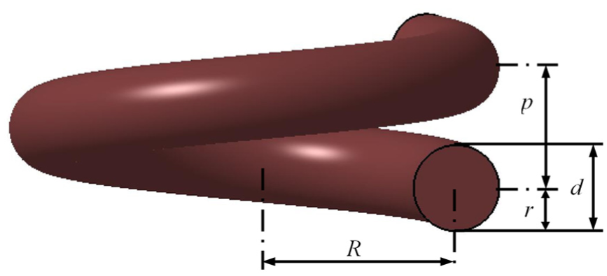
3D modeling of a helical pipe.

Table 1.

Details of cases analyzed.

Pipe no.	1	2	3	4	5	6	7
Coil pitch, p (mm)	75	0	75	75	75	95	150
Curvature radius, R (mm)	662.5	662.5	250	150	1500	662.5	662.5

Mesh and grid sensitivity analysis

The grids for the computational domains were generated by the meshing tool ICEM CFD with the blocking method. The grid details for the whole domain are shown in Figure 2. Five mesh schemes were used to prove the grid independence by simulating the flow field with different numbers of grid nodes in Table 2. Figure 3 illustrates the grid sensitivity analysis through axial velocity in x-direction along the circumference of cross-section at half length. The simulated axial velocity had a slight change when the grid number was more than 0.794 million, which indicated the calculation results tend to stable. Therefore, Mesh 4 was selected to be the final computing grid in consideration of the computation resource. The maximum non-dimensional wall distance y⁺ for the whole flow field was lower than 80, which satisfy the requirement of each turbulence modeling method adopted in this article.

Figure 2.

Computational grid.

Table 2.

Mesh schemes.

Scheme	Mesh 1	Mesh 2	Mesh 3	Mesh 4	Mesh 5
Number of grids	248,368	422,608	683,064	794,760	991,968

Figure 3.

Grid sensitivity analysis.

Boundary conditions

In the steady state simulation, governing equations are solved in a stationary framework. Water at 25° was chosen as the working fluid, with the reference pressure of 1 atm. The uniform axial speed was specified at the inlet and the outlet boundary was set as opening with a relative static pressure value of zero. A no-slip wall condition was imposed on the physical surface of the helical pipe. The convergence criterion was set to 10⁻⁵. The high-resolution scheme was used for the discretization of advection term and diffusion term. The fully implicit multi-grid coupled algorithm was used to solve all the hydrodynamic equations as a single system.

Turbulence model

Four turbulence models including standard k-ε model, re-normalization group (RNG) k-ε model, SST k-ω model, and k-ω model were selected to carry out the numerical calculations. Figure 4 shows the comparison of both test and numerical results with different turbulence models for the value of friction factor. The result of SST k-ω model was closest to the test data, which had an average deviation of 1.7%. Piazza and Ciofalo¹⁷ also showed that SST k-ω model was better in prediction of flow characteristic in helical pipe as compared to standard k-ε model. Therefore, the SST turbulence model was used in numerical computation. This model was developed by Menter,²⁴ combining advantages of both the standard k-ε model and the standard k-ω model. It automatically switched to the k-ω model in the near region and the Standard k-ε Model away from the walls.

Figure 4.

Numerical results with different turbulence models.

Results and discussion

Validation of numerical codes

The experiment was performed in an open test bed, as shown in Figure 5(a). It contains the following components: a polyethylene (PE) helical pipe, a centrifugal pump, a flowmeter, a set of pressure gauges, two valves, and a pipeline. The mass flow was measured by an electromagnetic flowmeter with an estimated experimental uncertainty of 0.5%, which was installed between the outlet of the centrifugal pump and the inlet of the PE helical pipe. Pressure measuring points were, respectively, located at the inlet and outlet of both the PE helical pipe and the centrifugal pump. In order to reduce the impact of secondary flow in measurement of pressure, measurement devices were installed at the inlet and outlet of the PE helical pipe in Figure 5(b). The measurement device was consisted of a connecting pipe, a piezometer ring, and a pressure gauge connector. The water flowed from the connecting pipe to the piezometer ring by four guiding pressure holes evenly distributed in the connecting pipe wall along the circumference. The piezometer ring was installed at 2d away from the outlet of the PE pipe, using to connect the pressure gauge. Water was sucked from an open reservoir by the centrifugal pump, and then flowed back the reservoir through the PE helical pipe. The valve at outlet of the centrifugal pump was used to control the flow rate.

Figure 5.

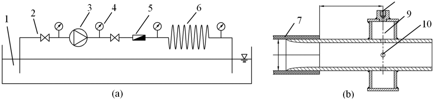
The experimental setup: (a) open test rig and (b) device of acquiring pressure.

Ito²⁵ and Murakami et al.²⁶ correlations are most widely accepted for single-phase pressure drop in curved pipe for turbulent flow, as equations (1) and (2), defining the variable f_c representing the friction factor of helical pipe. The Fanning friction factor^27,28 contributes to pressure drop (Δp) served as the variable compared with numerical simulation for empirical calculations, which is defined by equation (3)

f_{c} = \frac{1}{4} {(\frac{r}{R})}^{\frac{1}{2}} {0.029 + 0.304 {[R e {(r / R)}^{2}]}^{1 / 4}}

(1)

f_{c} = {[R e {(\frac{r}{R})}^{2}]}^{1 / 20} \times 0.079 R e^{- 0.25}

(2)

Δ p = \frac{2 f_{c} ρ u^{2} L}{d}

(3)

where u is the velocity, and variables L and d are described as the length and the diameter of the pipe, respectively.

Experimental data and two empirical calculations were collected to compare with numerical simulated results for pressure losses in pipe 1. Figure 6 shows an acceptable agreement with experimental data and empirical calculation. Experimental data at the flow rate ranging from 10 to 40 m³/h are almost consistent with numerical results. The maximum deviation between the simulated results and experimental values of the pressure drop is 2.9%. The mean deviations between two empirical calculations and the numerical result are lower than 5%. The maximum deviations between two empirical calculations and the numerical result are 9% and 5.3%, respectively. Therefore, it is certain that the numerical computational method used in this study is correctly implemented, and new simulation can be conducted at different values of De, curvature radius, and coil pitch.

Figure 6.

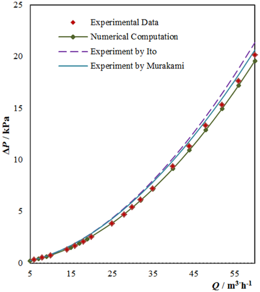
Comparison of predicted, measured, and empirical results.

Developments of velocity and pressure distributions at different angular positions

Velocity and pressure distribution at various planes along the length of pipe 1 were numerical simulated to analyze the flow structure inside the helical pipe. Figure 7(a) presents an overview of velocity contours for various cross-sections along the pipe 1 and the details at some typical cross-sections are specified in Figure 7(b). The sectional planes are identified by the angle θ from 0° to 360°, starting from the pipe inlet (θ = 0°), and the subsequent planes are 10° apart in Figure 7(a).

Figure 7.

Velocity contours at (a) various plans and (b) selected plans along the length coil.

Up to the angle of 60°, the maximum velocity in the pipe was found to increase gradually. Subsequently, the velocity profile at the cross-section was symmetric and the area of high velocity region reduced as the flow develops. This behavior led to the increase in the velocity gradient in the cross-section and contributed to unsteady flow along the length of helical pipe.

To analyze the pressure distribution of inner helical pipe, a dimensionless pressure coefficient C_p is defined as follows

C p = \frac{p - p_{r e f}}{(1 / 2) ρ u^{2}}

(4)

where p_ref is the average pressure and u is the mean velocity for the inlet plane of helical pipe.

The pressure drop in helical pipe was observed downstream from the angle 0° to 360° in Figure 8(a). According to the above analysis of the velocity distribution, the pressure energy of fluid is transformed into the kinetic energy along the pipe. Figure 8(b) presents the pressure distribution in the circumference of the cross-sections of the angle 0°, 45°, 90°, 135°, 180°, 225°, 270°, 315°, and 360°. It is shown that the variation pressure is predominant in the central region of each cross-section circumference. The differences in pressure in both sides of the sectional plane transversal led to obvious pressure gradient along the same direction. The water flowed to the pipe ektexine with the bigger curvature radius under the influence of the syphon, resulting in squeeze flow. The squeeze flow produced pressure difference in the cross-section. Obviously, large pressure differences observed in the angle of 180° and 315° cross-section illustrated the large force generated on the pipe ektexine locations of both angles. The large force was one of the main causes to induce the pipe deformation.

Figure 8.

Pressure coefficient distribution (a) in the equatorial mid-plane and (b) along the circumference of selected cross-sections.

Although the above obvious velocity and pressure variations can be noticed along the length of the helical pipe, the flow pattern cannot be easily indicated specifically in this way. Therefore, the numerical simulating streamline method will be used for this case, and the results will be discussed in the next section.

Comparison of streamline patterns for different pipe parameters

The helical pipe parameters, including the De, the coil pitch, and the curvature radius, play an important role in flow structure inside the pipe. Based on the pipes 1–3, the effects of these factors on flow characteristics were analyzed by predicting streamlines as shown in Figure 9(a)–(c). The secondary flow was visualized by illuminating numerical simulating streamlines in cross-sections. The streamline curves of double vortices were symmetrical about the horizontal diameter of each cross-section. In Figure 9(a), the centers of double vortices shift toward the upper wall symmetrically with the gradual increase in the De. Such alterations in the nature of the streamlines are noticeable when the De is larger than 200. Moreover, it can be seen that the streamline spacing is homogeneous in the high De pipe, while the kinetic energy loss in flow structure of low De pipe is stronger than that of high De pipe. Figure 9(b) shows that the vortex center takes a slight deflection and the flow is seemed to be concentrated in the vortex center with the increase in the coil pitch. The coil pitch influences mainly on the rotational position of secondary vortices around its longitudinal axis. In Figure 9(c), the vortex center shifts toward the upper wall slightly when the curvature radius reduces drastically. Thus, the effects of the De and the coil pitch on the secondary flow within the helical pipe are quite significant.

Figure 9.

Variation of streamlines on the 180° plane for (a) different Dean numbers, (b) different coil pitches, and (c) different curvature radiuses.

Comparison of friction factor

The friction factor is the major factor representing the flow loss extent in the helical pipe, while the secondary flow results in the flow loss. Considering the effects of the helical pipe parameters, containing the De, the curvature radius and the coil pitch, the friction factor was analyzed to account for the loss mechanism and law using pipe 1, pipes 3–7. Figure 10(a) presents that the friction factor drops enormously when the De increases from 10 to 100,000 under the constant coil pitch (p = 75 mm) by pipe 1, pipes 3–5. The friction factor decreases to some extent with the increase in the curvature radius from 150 to 1500 mm. Similarly, the friction factor reduces from 0.0075 to 0.0045 with the growth in the De from 5000 to 50,000 with constant curvature radius (R = 662.5 mm) by pipe 1, pipe 6, and pipe 7, as shown in Figure 10(b). The pipe with the bigger coil pitch has the smaller friction factor, that is, the pipe has less flow losses. Therefore, adding the values of the curvature radius and the coil pitch can diminish the friction factor to reduce flow losses within the helical pipe.

Figure 10.

Friction factors versus Dean numbers among (a) different curvature radiuses and (b) different coil pitches.

Conclusion

Flow characteristics within the helical pipe were presented by CFD calculation in this article. The numerical methodology was validated by comparing with the results of the experimental and empirical mathematical calculations. The maximum deviation between the experimental values and the simulated results of the pressure drop is just 2.9%.

The velocity and pressure distributions within the helical pipe were predicted along the length of the pipe. The maximum velocity increases along the pipe gradually and forms a large gradient field in the cross-section to cause unsteady flow in the pipe. Conversely, the pressure reduces along the pipe and large pressure differences observed in the angle of 180° and 315° cross-section generate the corresponding centrifugal forces on the helical pipe, due to the squeeze flow.

The secondary flow was presented obviously by illuminating streamlines. The double vortices are symmetrical about the horizontal diameter of each cross-section. The effects of the helical pipe parameters on the secondary flow were explored. The vortex center shifts toward the upper wall with the increase in the De. The vortex center takes a slight deflection with the increase in the coil pitch.

The friction factor was studied to account for the loss mechanism by altering the helical pipe parameters. The increases in the curvature radius and the coil pitch can diminish the friction factor to reduce flow losses within the helical pipe.

Footnotes

Academic Editor: Pietro Scandura

Declaration of conflicting interests

The author(s) declared no potential conflicts of interest with respect to the research, authorship, and/or publication of this article.

Funding

The author(s) disclosed receipt of the following financial support for the research, authorship, and/or publication of this article: This research was supported by the National Key Research Program (No. 2016YFC0400104), National Studying Abroad Foundation of China, and Graduate Student Innovation Projects of Jiangsu Province (Grant No. CXLX13_660).

References

Eustice

Experiments on stream-line motion in curved pipes. P R Soc Lond A: Conta 1911; 85: 131–199.

Dean

WR.

Note on the motion of fluid in a curved pipe. Philos Mag 1927; 4: 208–233.

Truesdell

Jr Adler

RJ.

Numerical treatment of fully developed laminar flow in helically coiled tubes. AIChE J 1970; 16: 1010–1015.

Akiyama

Cheng

KC.

Boundary vorticity method for laminar forced convection heat transfer in curved pipes. Int J Heat Mass Tran 1971; 14: 1659–1675.

Austin

Seader

JD.

Fully developed viscous flow in coiled circular pipes. AIChE J 1973; 19: 85–94.

Wang

CY.

On the low-Reynolds-number flow in a helical pipe. J Fluid Mech 1981; 108: 185–194.

Germano

The Dean equations extended to a helical pipe flow. J Fluid Mech 1989; 203: 289–305.

Cioncolini

Santini

An experimental investigation regarding the laminar to turbulent flow transition in helically coiled pipes. Exp Therm Fluid Sci 2006; 30: 367–380.

Hayamizu

Yamamoto

Yanase

Experimental study of the flow in helical circular pipes: torsion effect on the flow velocity and turbulence. J Therm Sci 2008; 17: 193–198.

10.

Gupta

Wanchoo

Jafar Ali

TRM

. Laminar flow in helical coils: a parameter study. Ind Eng Chem Res 2011; 50: 1150–1157.

11.

Pimenta

Campos

JBLM

. Friction losses of Newtonian and non-Newtonian fluids flowing in laminar regime in a helical coil. Exp Therm Fluid Sci 2012; 36: 194–204.

12.

Amicis

Cammi

Colombo

LPM

. Experimental and numerical study of the laminar flow in helically coiled pipes. Prog Nucl Energ 2014; 75: 206–215.

13.

Mandal

Nigam

KDP

. Experimental study on pressure drop and heat transfer of turbulent flow in tube helical heat exchanger. Ind Eng Chem Res 2009; 48: 9318–9324.

14.

Hardik

Baburajan

Prabhu

SV.

Local heat transfer coefficient in helical coils with single phase flow. Int J Heat Mass Tran 2015; 89: 522–538.

15.

Kim

Son

An experimental study on the pressure drop and heat transfer through straight and curved small diameter tubes. J Mech Sci Technol 2014; 28: 797–809.

16.

Kim

Choi

CY.

Numerical simulation of subcooled flow boiling heat transfer in helical tubes. J Press Vess: T ASME 2009; 131: 011305 (9 pp.).

17.

Piazza

Ciofalo

Numerical prediction of turbulent flow and heat transfer in helically coiled pipes. Int J Therm Sci 2010; 49: 653–663.

18.

Jayakumar

Mahajani

Mandal

JC.

CFD analysis of single-phase flows inside helically coiled tubes. Comput Chem Eng 2010; 34: 430–446.

19.

Malheiro

Oliveira

Pinho

FT.

Parametric study on the three-dimensional distribution of velocity of a FENE-CR fluid flow through a curved channel. J Non-Newton Fluid 2013; 200: 88–102.

20.

Noorani

Khoury

GKE

Schlatter

Evolution of turbulence characteristics from straight to curved pipes. Int J Heat Fluid Fl 2013; 41: 16–26.

21.

Pan

Zhou

Wang

CFD study of heat transfer foe oscillating flow in helically coiled tube heat-exchanger. Comput Chem Eng 2014; 69: 59–65.

22.

Nobari

MRH

Kazemi

Nourian

A numerical investigation of incompressible viscous flow in a helical square annulus. Appl Math Comput 2016; 277: 127–141.

23.

Kang

Yang

K-S.

Large eddy simulation of turbulent heat transfer in curved-pipe flow. J Heat Transf: T ASME 2016; 138: 011704 (11 pp.).

24.

Menter

FR.

Two-equation eddy-viscosity turbulence models for engineering applications. AIAA J 1994; 32: 269–289.

25.

Ito

Friction factors for turbulence flow in curved pipes. Trans Am Soc Mech Eng 1959; 81: 123–134.

26.

Murakami

Mori

Sano

A study on the hydraulic loss of tubular coils. B JSME 1971; 14: 1296–1303.

27.

Oertel

Prandtl—FÜhrer durch die StrÖmungslehre, vol. 11. Auflage, Friedr Vieweg & Sohn Verlagsgesellschaft, Wiesbaden, 2002.

28.

Mishra