
Abstract
Bridges are vulnerable to the fatigue damage accumulation caused by traffic loading over the service period. A continuous growth in both the vehicle weight and the traffic volume may cause a safety hazard to existing bridges. This study presented a computational framework for probabilistic modeling of the fatigue damage accumulation of short to medium span bridges under actual traffic loading. Stochastic truck-load models were simulated based on site-specific weigh-in-motion measurements. A response surface method was utilized to substitute the time-consuming finite element model for an efficient computation. A case study of a simply supported bridge demonstrated the effectiveness of the computational framework. Numerical results show that the simulated fatigue stress spectrum captures the probability density functions of the heavy traffic loading. The equivalent fatigue stress range increases mostly linearly in the good road roughness condition with the growth of the gross vehicle weight. The vehicle type and the road roughness condition affect the stress range. The influence of the driving speed on the equivalent stress range is non-monotonic. The bridge fatigue reliability has a considerable increase even under a relatively high overload limit. It is anticipated that the proposed computational framework can be applied for more types of bridges.
Keywords
Introduction
With the steady growth of the global economy and the intense competition of the transportation market, the traffic loading on highway bridges has increased over the last decades.1,2 Such continuous increase in the traffic loading may pose a safety threat to the existing bridges. As a result, several bridges were collapsed due to couples of overloaded trucks.3,4 Fatigue damage induced by heavy trucks is one of these failure mechanisms as summarized by Deng et al. 5 leading to the collapse of in-service bridges. For the short to medium span bridges, the applications of the high strength materials, the design theory that makes full use of strength of materials in high stress condition, and the decreasing dead-to-live-load ratio make them fatigue-sensitive to vehicle loads. 6 Therefore, the traffic-load-induced fatigue damage accumulation of short to medium span bridge deserves investigation.
It is acknowledged that the bridge fatigue evaluation mainly involves two aspects including the structural resistance evaluation and the load effect computation. Great progresses have been made on investigations of the bridge fatigue behavior in recent years. Ma et al. 7 proposed a new crack-growth-based corrosion fatigue life prediction method for aging reinforced concrete (RC) beams. Characteristic stress-life (S-N) curves were proposed by Ghahremani et al. 8 for the fatigue design of treated welds under variable amplitude loading in the high cycle domain. In addition to the above-mentioned, the traffic loading is also a critical factor impacting the fatigue damage accumulation. In this regard, Zhang et al. 9 evaluated the fatigue reliability of long-span bridges under combined dynamic loads from winds and vehicles. Wang et al. 10 investigated the vehicle–bridge interaction of the fatigue stress range and the number of stress cycles of short-span bridges. The influence of different road roughness conditions (RRCs) and vehicle speeds of bridges on dynamic amplification factors (DAFs) of load effects was also been considered for fatigue design of existing bridges. 11 However, influence of the vehicle dynamic effect in conjunction with the traffic growth on the fatigue reliability of short to medium span bridges is still not clear.
It is acknowledged that the stress spectra of the bridge critical components are a precondition for fatigue reliability assessment. For the simulation of the stress spectra, in addition to the structural health monitoring (SHM) approach,12–14 the numerical simulation based on weigh-in-motion (WIM) measurements is an alternative method for a wide range of bridges. Due to the stress spectra being sensitive to site-specific traffic loads, numerous studies have been conducted to develop fatigue truck-load models based on site-specific WIM measurements. Typical fatigue truck-load models with deterministic configurations and gross vehicle weights (GVWs) have been specified or recommended in national design codes, such as AASHTO, 15 Eurocode 1, 16 and BS5400. 17 However, Zhou 18 indicated that fatigue analysis based on specification loads and distribution factors usually underestimates the remaining fatigue life of existing bridges by overestimating the live-load stress ranges. Chotickai and Bowman 19 found that fatigue damage can be notably overestimated in short-span girders utilizing the 240-kN AASHTO fatigue truck. The different research conclusions mentioned above illustrate the deterministic fatigue truck models in specifications cannot capture the characteristics of the local transportation as a result of an inaccurate fatigue analysis. For this reason, the randomness of vehicle parameters begins to be widely accepted in simulating the actual vehicle model. In this regard, Guo et al. 20 assessed the fatigue reliability of steel bridge details via integrating WIM data and probabilistic finite element analysis (FEA), which simulated the traffic condition vividly and made the uncertainties associated with vehicle parameters well considered. However, the axle weight in Guo’s truck model obeyed a standard Gaussian distribution that cannon reflect a multi-peaks feature of the actual traffic condition. Currently, most of the stochastic analysis on vehicle parameters is associated with estimation of DAF.21,22 Application of stochastic truck-load model to fatigue reliability assessment of short to medium span bridges is insufficient.
This study aims to present a computational framework for fatigue reliability evaluation of short to medium span bridges under stochastic truck loading. As the first task, the equivalent fatigue stress and the limit state function (LSF) of the short to medium span bridge under stochastic traffic loading are formulated. Subsequently, a framework is proposed to simulate the fatigue stress spectrum of the bridge under stochastic simulation more effectively. Finally, the proposed framework and the stochastic traffic loads are applied to a simply supported bridge. Influence of the stochastic parameters including the vehicle speed, the RRC, and the GVW on the stress range is investigated. The effect of traffic growth and an overload control on the fatigue reliability is emphasized.
Theoretical bases
Truck-induced fatigue damage accumulation
It is acknowledged that each truck passage will yield several stress blocks in the bridge structures. These stress blocks have the properties of high cycles and low amplitudes. In general, these stress blocks are converted to fatigue damage by the S-N approach. Several design codes have specified S-N curves for various structural details. Eurocode 3 16 is utilized herein to define the S-N curve. In Eurocode 3, the fatigue strength of nominal stress range is represented by a series of curves with respect to typical detail categories. The category is designated by the fatigue strength ΔσC at 2 million cycles. The S-N curve in Eurocode 3 is expressed as


where ΔσR is the stress range, NR is the number of cycles, ΔσD and ΔσL are constant-amplitude fatigue limit and fatigue threshold, respectively, and KC and KD are the fatigue strength coefficients with respect to ΔσR > ΔσD and ΔσR ≤ ΔσD, respectively. In this study, as the research objective, the steel bar in concrete bridges has a category of 80 MPa. Details of the parameters in the S-N curve are shown in Table 1.
Parameters of S-N curve in the Eurocode 3 specification.
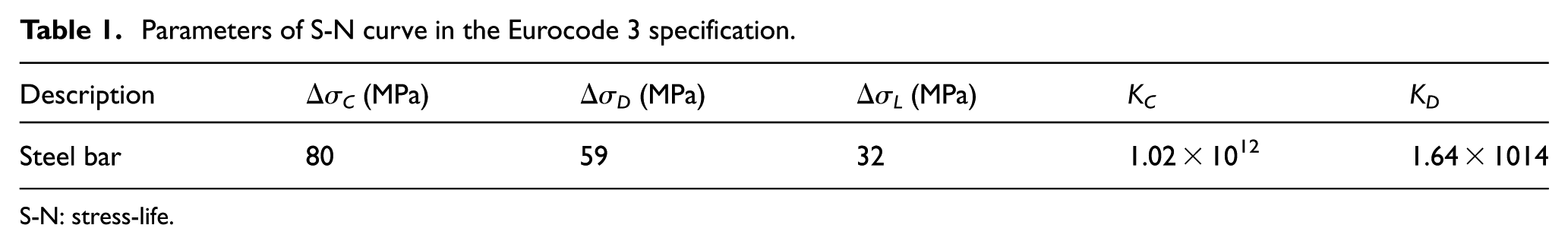
S-N: stress-life.
In addition to the S-N curve, the well-known Palmgren’s fatigue damage accumulation theory is a theoretical basis for the fatigue damage analysis as well. In Palmgren’s theory, 23 the fatigue damage caused by variant-amplitude stress cycles is linearly accumulated. By integrating the linear accumulation formula and the S-N curve, the structural fatigue damage accumulation is written as 15

where Δσi and Δσj are the ith and jth stress ranges that are larger than and less than ΔσD, respectively. Ni and Nj are the number of cycles of Δσi and Δσj, respectively.
Before utilizing the fatigue damage accumulation formula shown in equation (3), the variant-amplitude stress cycles should be converted into constant-amplitude stress cycles. The equivalent formula can be derived by equations (1)–(3) and is written as

where Δσre is the equivalent stress range.
Herein, the truck-induced fatigue damage accumulation can be obtained by implementing the S-N curves specified in Eurocode 3 and the linear accumulation criterion. The equivalent stress range caused by an individual truck passage can also be derived.
LSF of fatigue damage accumulation accounting for traffic growth
A LSF is to describe the relationship between fatigue resistance and fatigue loading, which is the basis for fatigue reliability evaluation. The LSF is essential for fatigue reliability evaluation taking into account the stochastic parameters in structural resistance and loading analysis. On this basis, the structural component will be demanded as fatigue failure when the number of stress cycles reaches a critical value. In this study, the major stochastic parameters, the GVWs and the traffic volume, are growing with the development of national economy and should be considered in the LSF. Assuming that the GVW increases linearly, the LSF of fatigue damage accumulation during the lifetime of a bridge is written as 24
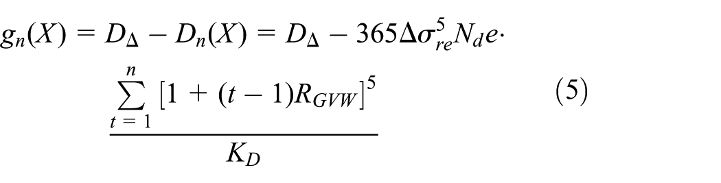
where gn(X) is the LSF of bridges in the nth year, X is a random variable, DΔ is the Miner’s critical damage accumulation index, Dn(X) is the cumulative fatigue damage in the nth year, e is the distribution coefficient of transverse axle load, Nd is the number of daily cycles with respect to Δσre, and RGVW is the annual linear growth rate of the GVW.
With the explicit expression of the LSF shown in equation (5), an appropriate approach can be selected to conduct an accurate fatigue reliability evaluation. Monte Carlo simulation (MCS) 25 is utilized herein to calculate the fatigue reliability of the LSF. Suppose that the sample size be N, the estimation of failure probability is described as

where I(Ai) is a characteristic function; I(Ai) = 1, if the function value is less than 0, otherwise I(Ai) = 0. According to the geometric meaning of reliability index, the relationship between reliability index and failure probability can be described as

where norminv represents the inverse function of a normal distribution function. Herein, fatigue reliability of bridges under site-specific stochastic loading accounting for the growth of traffic can be calculated with the application of the proposed LSF and MCS.
Proposed computational framework for stress spectrum modeling
Conventional approaches
The stress spectrum depends on the geometry of the vehicles, the axle loads, the vehicle spacing, the composition of the traffic, and its dynamic effects. In this regard, various fatigue load models (FLMs) were defined in the national design specifications.15–17 Taking Eurocode 1 16 as an example, five FLMs were defined here to calculate the stress spectrum for different applications. FLM 1 has the configuration of the characteristic of load model 1 defined in 4.3.2 of Eurocode 1. FLM 2 consists of a set of idealized lorries. FLM 3 was defined as single vehicle model, which consists of four axles, each of them having two identical wheels. The geometry of FLM 3 is shown in Figure 1. The weight of each axle is equal to 120 kN, and the contact surface of each wheel is a square of side 0.40 m. FLM 4 consists of sets of standard lorries, which together produce effects equivalent to those of typical traffic on European roads. FLM 5 consists of the direct application of recorded traffic data, supplemented, if relevant, by appropriate statistical and projected extrapolations. In the above categories, FLMs 3, 4, and 5 are intended to be used for the fatigue life assessment by reference to fatigue strength curves defined in EN 1992 to 1999. With these FLMs, there are three procedures for stress spectrum molding: (1) conduct the finite element simulation of a bridge under typical fatigue truck-load model and extract the stress histories; (2) extract stress cycles via rainflow counting method; 26 (3) calculate structural fatigue damage based on Palmgren–Miner criterion. In the above content, the establishment of typical fatigue truck-load model is of crucial importance.

Fatigue load model 3 in Eurocode 1.
As mentioned above, the typical fatigue truck-load model is able to conduct a deterministic estimation of the fatigue condition of bridges. However, as shown in the introduction, the deterministic analysis cannot reflect the probability characteristic of the traffic condition for an accurate fatigue reliability assessment of bridges.
The proposed computational framework
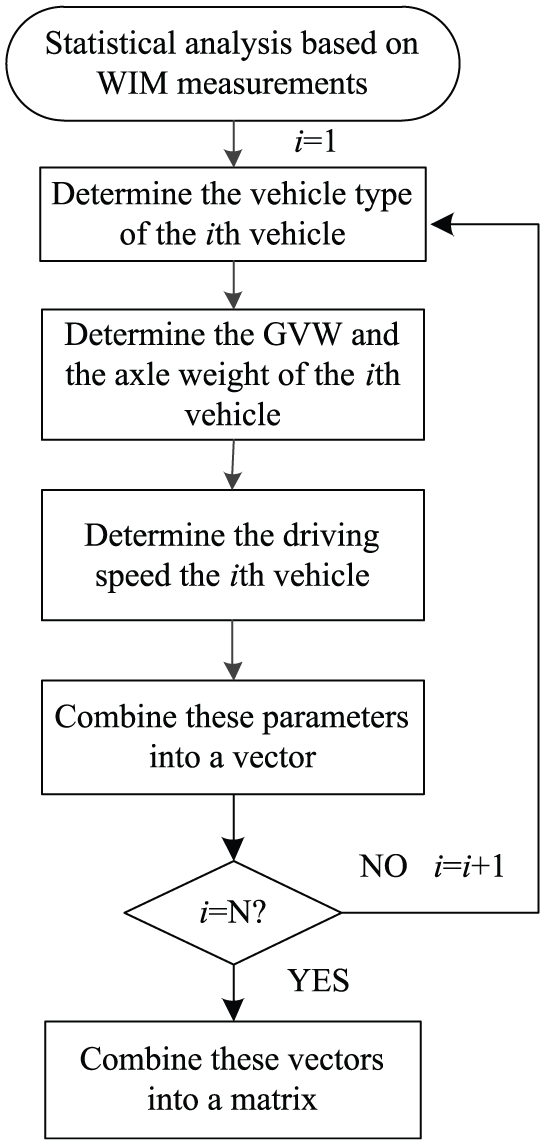
For the aforementioned problems, a stochastic fatigue truck-load model based on site-specific WIM measurements is developed here to replace the typical fatigue truck-load model for the fatigue reliability estimation. A stochastic truck-load model is a parametric truck-load model integrated with statistic parameters, such as the GVWs, the vehicle types, the driving lanes, and the vehicle speeds. The stochastic truck-load model can be simulated in the time domain. If the conventional approach is utilized to simulate the stress spectra under the stochastic truck-load model, the traffic volume of thousands of vehicles per day need huge computational efforts. Therefore, in order to solve the time-consuming problem, a response surface method (RSM) is utilized herein to approximate the function relationship between vehicle parameters and structural fatigue stress range. The RSM can reflect the structural fatigue stress under the stochastic truck-load model with a small number of samples for finite element program runs. The flowchart of the computational framework is shown in Figure 2.
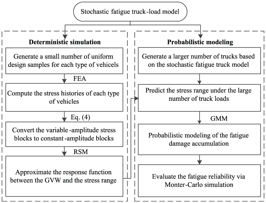
Flowchart of the proposed computational framework.
As shown in Figure 2, there are two critical steps including the deterministic simulation and the probabilistic modeling of damage accumulation. The deterministic simulation is to approximate response surface function based on a small number of truck samples. The probabilistic modeling is to conduct a probabilistic analysis of fatigue damage accumulation.
Probabilistic modeling of fatigue load effects is a significant procedure for the structural fatigue reliability evaluation. The probabilistic distribution of fatigue analysis was discussed initially by the American Society of Civil Engineers (ASCE) Committee on Fatigue and Fracture Reliability. 27 Subsequently, distributions of Weibull, Beta, and Lognormal for loading were utilized to calculate equivalent stress range. In this regard, Pourzeynali and Datta 28 utilized Lognormal and Weibull distributions to analyze fatigue reliability of suspension bridges. Guo et al. 20 utilized the normal and Lognormal distribution models to simulate the vehicle parameters including the axle weight and axle spacing based on the WIM measurements monitored from 2005 and then various stress ranges in fatigue critical components. However, the increasingly heavy-duty trucks in recent years lead to the complication of simulating the fatigue load effects via a standard probability distribution model. Xia et al. 29 characterized the multi-load effects such as traffic and wind with the application of the mixture distribution models. Similarly, Gaussian mixture model (GMM), 30 a method with ability to approximate the density distribution of any arbitrary shape smoothly, is utilized to capture the multi-peak distribution characteristics in this study. The procedures of the GMM are as follows: (1) analyze the likelihood function between monitoring data of fatigue loading; (2) develop iterative estimations of parameters in the GMM including weight, mean value, and variance with the utilization of expectation-maximum algorithm; (3) determine the optimal GMM probability model based on Akaike information criterion (AIC) and the Bayesian information criterion (BIC). 31 The probability density function (PDF) of a GMM is written as

where ai, µi, and σi are the weight, mean value, and variance of the ith variable in GMM, respectively, and M is the number of Gaussian models.
A finite element run is essential for each truck passage. It is a time-consuming computation for the entire truck samples in the stochastic truck-load model. Therefore, the machine learning 32 was applied herein for effective operation through devising complex models and algorithms that lend themselves to prediction. In general, machine learning approaches mainly include the neural network method (NNM), the support vector machine (SVM), the interpolation function method (IFM), and the RSM. In this regard, the selection of an appropriate method is particularly important. These methods have their own characteristics. The NNM requires massive parameters and has an over-fitting problem. The SVM requires larger sample inputs and has no general solution for nonlinear problems, and the IFM with linear relation between two adjacent interpolation points is difficult to describe nonlinear phenomena. Therefore, the RSM,33,34 an optimization method with capability of solving the optimization of the time-consuming and nonsmooth problems, was selected herein to make the computation more efficient.
The RSM is a statistical and mathematical technique utilized to dispose the conversion problem between input and output in a complex system. A performance function with an explicit representation of random variables can be approximated by the regression of an analytical expression to replace the real surface function. A second-order RSM,35,36 the approximate function between vehicle parameters and Δσre is written as

where X is a random variable representing GVW in this study, g(X) is the structural performance function, and a, b, and c are coefficients that will be approximated by the training data. It is worth noting that a response surface function of vehicle of type Vi can be approximated by 2i + 1 times of computer runs.
Stochastic fatigue truck-load simulation
An accurate simulation of the stochastic fatigue truck-load model is the precondition of fatigue assessment. One or few simple distributions without a comprehensive consideration of the random characteristics will contribute to large errors in fatigue evaluation. For fatigue analysis of bridges, the application of stochastic truck-load model with time-variant characteristic has great important significance. The stochastic traffic flow is a probability model that takes relevant parameters as random variables. These parameters mainly include the vehicle configuration, the GVW, the vehicle spacing, and the driving speed. The vehicle configurations and the GVW are directly relative to the number of stress cycles and stress ranges, which affect the calculation of fatigue damage shown in the aforementioned LSF. Therefore, these two factors are considered in this study. As the study objects herein are small to medium span bridges, it is a small probability event that two cars travel on the bridge at the same time. Therefore, the influence of vehicle spacing is ignored. A flowchart of the framework for stochastic fatigue truck-load simulation is shown in Figure 3.
Flowchart of the stochastic fatigue truck-load simulation.
The statistical analysis of traffic flows can be estimated based on the site-specific WIM measurements. With the statistical database, the stochastic fatigue truck-load model can be generated via MCS. According to the framework, the first step is to generate the vehicle type. Subsequently, generate the GVW and the axle weight, respectively. At last, determine the driving speed of the corresponding vehicle. Herein, a vector of the ith vehicle type is obtained with the combination of the aforementioned parameters. Finally, the traffic matrix can be obtained by repeating the above steps. It is worth noting that the almost linear relationship between the axle weights and the GVW of the corresponding vehicle type was utilized to make the statistics of the axle weight more authentic.
Case study
The simply supported prestressed T-beam bridge is chosen here as prototype to demonstrate the effectiveness and application of the stochastic fatigue truck-load model and the computational framework for fatigue reliability assessment.
Bridge details and traffic loading
The widely used simply supported bridge with T-girders is selected as a case study to demonstrate the proposed computational framework. Dimensions of the cross section at the central point of the girder (L = 40 m) are shown in Figure 4. The fatigue critical components are the steel bars at the bottom of the cross section. Normally, the prestressed girders will not crack in the lifetime, except for undeserved or unsuitable construction or operation in the bridge lifetime. Once the concrete of the girder cracks, the stress of the steel bar will increase and has a risk of fatigue damage.

Dimensions of the cross section at the middle of a girder of the bridge with L = 40 m.
WIM measurements of a highway bridge in Sichuan, China, are utilized in this study. Details of the relevant data can be found in the work by Liu et al. 37 As the research objective is the heavy vehicles, filtering processes were conducted for the purpose of removing the invalid measurements. The measurements were excluded while meeting the following criteria: (1) the GVW is less than 30 kN; (2) the axle weight is greater than 200 kN or less than 5 kN; (3) the vehicle length is more than 20 m or less than 3 m; and (4) measuring data were affected by system error. The rest of vehicle samples were classified into six categories according to the vehicle configuration, where V1 represents the light cars and V2–V6 represent 2–6 axle trucks, respectively. Proportion of the vehicle types is shown in Figure 5. Subsequently, the PDFs of the GVWs of the relevant vehicle types were simulated via GMM based on the WIM measurements, as shown in Figure 6.
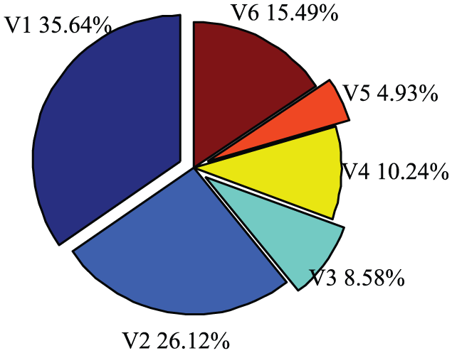
Proportion of vehicle types.

Probability density curves of GVWs of statistical trucks: (a) light truck, (b) two-axle truck, (c) three-axle truck, (d) four-axle truck, (e) five-axle truck, and (f) six-axle truck.
It is observed from Figures 5 and 6 that the heavy trucks have a high proportion and a high overload ratio in the actual traffic condition. GVWs of the highway have a significant characteristic of multi-modal distribution, which has been approximated by the multi-parameter GMM.
In accordance with the above statistics, stochastic truck-load model can be obtained within 1 h via the MCS based on the flowchart shown in Figure 3, as shown in Figure 7.
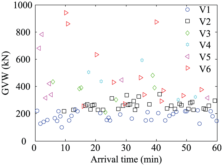
Simulated stochastic truck-load models.
As observed from Figure 7, each symbol indicates an individual truck. Even though these trucks are different from each other, they follow a prescribed probability distribution.
The simulation of the stochastic truck-load model indicates the accomplishment of the procedures in Figure 3. The statistical vehicle parameters including the vehicle type and the GVW provide the data basis for the subsequent simulation of stress spectra.
Probabilistic modeling of the fatigue stress spectrum
For fatigue damage analysis of the bridge under the simulated stochastic truck-load model, the dynamic impact was considered in the transient analysis. The RRC has a significant influence on the vehicle–bridge interaction. It is usually simulated by an inverse Fourier transformation and an assumed power spectral density. 22 The road roughness coefficients referred to the International Organization for Standardization (ISO) specification 38 for “Good,”“Average,” and “Poor” conditions are 32 × 10−6, 128 × 10−6, and 512 × 10−6 m3/cycle, respectively. In the finite element model, the load step is 0.01 s, the vehicle velocity is 20 m/s, the GVW of the vehicle is 100 kN, and the road roughness is supposed as “Good.” In order to study the influence of the vehicle spacing, which is the vehicle gap between two adjacent vehicles in the same lane, the vehicle spacing is supposed to be 20, 40, and 80 m on the stress history. The bridge with a span length of 40 m is selected herein as the objective. The computed results are shown in Figure 8.

Stress–time histories of a 40-m-length bridge under two adjacent three-axle truck loadings in different vehicle spacing.
It is worth noting that the vehicle spacing impacts the stress ranges of the bridge. The case of simultaneous presence of two vehicles on a bridge can be considered in two cases: (1) longitudinal direction in a same traffic lane; (2) transverse direction in different traffic lanes. For the first case, influence of the vehicle spacing in a traffic lane on the stress history was analyzed and shown in Figure 8. It is indeed observed that two vehicles with vehicle spacing of 20 m produce higher stress amplitude than the other two cases. Therefore, the vehicle spacing less than the bridge length will magnify the stress range. The simultaneous presence of two vehicles in the same traffic lane on a short to medium span bridge is relatively rare. Therefore, this study ignored vehicle spacing and supposed the vehicle crossed the bridge independently. Lu et al. 24 utilized a truck-by-truck simulation to conduct the stress spectrum simulation of an orthotropic steel bridge deck since most effective influence line is in the region between two diaphragms (3.2 m). The present objective is the simply supported girder bridge that is different to the steel bridge. Nevertheless, the length of the effective influence line of the simply supported bridge is much short than the regular vehicle spacing of highway bridges. For the second case, in the opening literature, the simultaneous presence of vehicles on a bridge is usually considered by a multiple presence factor (MPF). The practice specifications have defined the MPFs for different number of traffic lanes. For instance, the MPFs for the three traffic lanes are 0.85 and 0.75 according to the AASHTO 15 and the China’s code, respectively. Fu et al. 39 used WIM truck data to calibrate the code-specified MPF values, which were verified of being 400% higher than the practical case.
On the basis of these time–stress histories, the fatigue stress blocks can be estimated by the rainflow counting method. The RSM is utilized to approximate the function corresponding to each vehicle type between GVWs and Δσre. Taking the three-axle truck as an example, the approximated response function is

where w is GVW of each 3-axel truck.
In order to investigate the influence of the vehicle type and the RRC on the equivalent stress, suppose that a two-axle truck and a six-axle truck with GVWs between 20 and 120 t cross the bridge at a constant speed of 15 m/s. Their stress histories were evaluated based on the vehicle–bridge coupled vibration system. 22 The equivalent fatigue stresses of the bottom steel bar under various load cases are plotted in Figure 9. It is observed that the equivalent fatigue stress range increases mostly linearly for a good RRC with the growth of the GVW. In addition, the vehicle type and the RRC affect the stress range under the same GVW, where the vehicle with fewer axles and the worse RRC leads to higher stress ranges. These results demonstrate the significance of the fatigue stress calculation of short-span bridges accounting for the vehicle type and the RRC.

Influence of the GVW, RRC, and vehicle types on the equivalent stress range.
In addition to the vehicle type, the RRC, and the GVW, the driving speed of a vehicle influences the vehicle–bridge interaction. Suppose a six-axle truck with the GVW between 300 and 1500 kN and the driving speed between 60 and 120 km/h cross the bridge, the equivalent stress range versus the driving speed is not monotonous, as shown in Figure 10. Therefore, the influence of the driving speed on the equivalent stress range is a wave factor.

Response surface of the equivalent stress ranges associated with driving speeds and GVWs.
A total number of six response functions corresponding to six types of vehicles were fitted by 37 times of computer runs. However, without the RSM, the stress spectrum modeling with thousands of truck samples will cause an incredible number of computations with the consideration of dynamic impacts.
With the approximate response functions, the probabilistic modeling was conducted with the large number of simulated stochastic truck-load samples. The PDF of the equivalent stress range was fitted by GMM. In addition, the FLM 3 shown in Figure 1, as one of the models recommended in Eurocode 1, was taken as an example to estimate the corresponding equivalent stress range in Figure 11 for comparison between the stochastic truck-load model and the deterministic FLM in specification. Therefore, histograms and PDFs of the equivalent stress range and the number of daily cycles are shown in Figure 11.

Histogram and PDF: (a) equivalent stress range and (b) the number of daily cycles.
As shown in Figure 11(a), the equivalent stress range, a deterministic value of 26.45 MPa, calculated based on the FLM 3 cannot capture the characteristic of the GVWs of the actual traffic with large occupancy ratio of heavy-duty trucks and as a result of inaccurate fatigue assessment. For equivalent stress ranges based on the stochastic truck-load model, the two peaks in the histograms were well simulated by the multi-parameter GMM to describe the light and heavy loading states of trucks traveling on the bridge, which can also be demonstrated via the peaks of GVWs shown in Figure 6.
The probabilistic modeling of the fatigue stress spectrum indicates the accomplishment of the most of procedures in Figure 2, and the characteristics of the vehicle type and the GVW were well captured in the form of stress spectra for the subsequent fatigue reliability.
Fatigue reliability assessment
One of the applications of the probabilistic model illustrated above is the fatigue reliability evaluation. This can be achieved by utilizing the LSF shown in equation (5). The random variable X in the LSF is associated with five parameters including the equivalent stress range Δσre, the number of cycles Nd, the critical fatigue damage Δ, the transverse distribution coefficient of wheel load e, and the fatigue strength coefficient KD. Statistics of these random variables are shown in Table 2, where the statistics of the Δ and e are referred to Wirsching 40 and Lu et al. 24
Statistics of random variables.
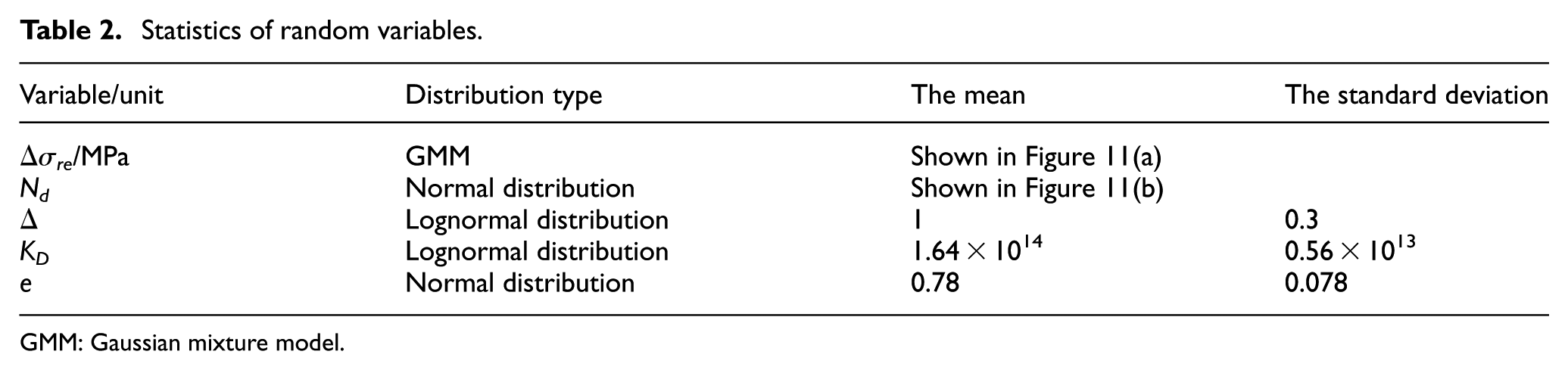
GMM: Gaussian mixture model.
With the statistics and the LSF, MCS is utilized to evaluate the failure probability of the bridge in lifetime. The fatigue reliability indices of simply supported T beams with span of 30 and 40 m have been evaluated without consideration of the growth of GVW. In the service lifetime of 100 years, the fatigue reliability index of the prototype bridges is shown in Figure 12. As observed from Figure 12, the fatigue reliability index of the 40-m-span bridge decreases to 2.74 in the 100 years, while the reliability index of 30-m-span bridge decreases to 4.68. It is obvious that the reliability index of the bridge with L = 40 m is much lower than that of the bridge with L = 30 m. The following investigation focuses on the bridge with L = 40 m.

Lifetime fatigue reliability indices of two simply supported bridges.
In practice, the traffic volume and GVW will increase with the development of global economy. This study assumes the annual linear growth rate of GVW, RGVW, to be 0%, 0.2%, 0.4%, and 0.6%. Based on this assumption, the fatigue reliability index of the 40-m-span bridge is evaluated. Figure 13 plots the influence of the RGVW on the fatigue reliability index. It is observed that the fatigue reliability index declines rapidly with an increase in the RGVW. This phenomenon can be explained by the LSF shown in equation (5), where the RGVW has a fifth power of impact on the fatigue damage accumulation.

Influence of GVW growth ratio on the fatigue reliability index.
In order to analyze the influence of the overload ratio on the fatigue reliability index of the prototype bridge, the overloaded trucks were excluded for a comparison. The specified weights corresponding to V2–V6 trucks are 20, 30, 40, 50, and 55 t, respectively, according to safe weight limits of bridges designed by current specifications in China. 41 Therefore, influence of the threshold overload ratio on the fatigue reliability index in the 100 years is evaluated under the different overload ratios and the annual linear growth rates, as shown in Figure 14.

Influence of threshold overload ratio on the fatigue reliability index.
As observed from Figure 14, the threshold overload ratio has a significant influence on the fatigue reliability. Even though the reliability index decreases with the growth of GVW, a strict threshold overload ratio can reduce the descent range. This result provides an effective way for the traffic management that the reasonable control of extremely overloaded truck can reduce the fatigue risk of existing bridges.
Conclusion
This study presented a method for evaluating fatigue reliability of short to medium span bridges based on site-specific stochastic traffic loading. The stochastic traffic was simulated by a fatigue truck-load model. A response surface function was utilized to make the deterministic simulation of fatigue stress more efficient. Application of the stochastic truck-load model and the computational framework was demonstrated through a case study of the simply supported bridge.
Numerical results of the case study show that the simulated fatigue stress spectra captured the PDFs of the heavy traffic loading, where the second peak of the stress spectrum is mostly caused by the overloaded vehicles. The equivalent fatigue stress range increases mostly linearly in the same RRC with the growth of the GVW, and the vehicle type and the RRC affect the stress range under the same GVW; the influence of the driving speed on the equivalent stress range is non-monotonic. As the annual linear growth rate of the GVW increases from 0% to 0.6%, the fatigue reliability index of the bridge decreases from 2.73 to 1.34. The bridge fatigue reliability has a considerable increase even under a relatively high threshold overload ratio. It is anticipated that the stochastic fatigue truck-load model and the proposed computational framework can be developed and applied for more types of bridges.
There are some challenges for further studies. First, the influence of the degradation of the road surface roughness condition should be considered as a more realistic vehicle–bridge interaction model. Second, the RSM can be replaced by the relatively developed machine learning approaches. Third, the influences of concrete cracking and reinforcement corrosion on fatigue damage should be considered. Finally, the traffic growth model should be more realistic rather than an annual linear growth factor. These shortcomings exposed in this study will be studied in the future work.
Footnotes
Appendix 1
Academic Editor: Eleni Chatzi
Declaration of conflicting interests
The author(s) declared no potential conflicts of interest with respect to the research, authorship, and/or publication of this article.
Funding
The author(s) disclosed receipt of the following financial support for the research, authorship, and/or publication of this article: This research was supported by the National Basic Research Program (973 program) of China (Grant No. 2015CB057706), the National Natural Science Foundation of China (Grant nos 51108046 and 51678068) Hunan Provincial Natural Science Foundation of China (Grant No. 13JJ6049), Science and Technology Project of Department of Communications of Guizhou Province (Grant No. 2014122019), Innovation Team Development Fund Project of Department of Education, Changsha University of Science and Technology (Grant No. 15QLTD04), the Open Fund of National Joint Engineering Research Laboratory for Long-term Performance Improvement Technology for Bridges in Southern China (CSUST Grant No. 16BCX02), and the Research Innovation Project of Graduate student in Hunan Province. Findings and conclusions expressed are those of the authors and do not necessarily represent the views of the sponsors.