
Abstract
This work presents the implementation in real-time of a neural identifier based on a recurrent high-order neural network which is trained with an extended Kalman filter–based training algorithm and an inverse optimal control applied to a tracked robot. The recurrent high-order neural network identifier is developed without the knowledge of the plant model or its parameters; on the other hand, the inverse optimal control is designed for tracking velocity references. This article includes simulation and real-time results, both using MATLAB®, and also the experimental tests use a modified HD2® Treaded ATR Tank Robot Platform with wireless communication.
Keywords
Introduction
A tracked robot is a mobile robot that runs on continuous tracks instead of wheels. The main advantage of a tracked robot is that it can be used to navigate in rough terrains.1,2
The thrust developed by a wheeled vehicle will generally be lower than that developed by a comparable tracked vehicle; 1 this is why these kinds of vehicles are used in a variety of applications where terrain conditions are difficult or unpredictable: urban reconnaissance, forestry, mining, agriculture, rescue mission scenarios, autonomous planetary explorations, to name but a few.2,3 Besides, tracked robots offer some other advantages, such as follows:
Tracked robots are versatile vehicles in different terrains and weather conditions.
Tracked robots generate low ground pressure which conserves the environment.
The design of tracked robots prevents them from sinking or becomes stuck into soft ground.
Tracked mobile robots can be considered as the most important type of mobile robots, and an extensive class of controllers has been proposed for trajectory tracking for this kind of robots;4–7 these works have the common characteristic that they need to know a lot of information about the system to be controlled and most of them are implemented in continuous time.
It is well known that the current trend towards digital rather than analogue control of dynamic systems is mainly due to the advantages found in working with digital rather than continuous-time signals. 8 This work is based on the previous work 9 where the recurrent high-order neural network (RHONN) identifier and an inverse optimal control scheme for all-terrain tracked robots are presented with just one simulation result. The RHONN is used to identify the plant model and it is trained with an extended Kalman filter (EKF)–based algorithm, under the assumption that the whole state is available for measurement. On the other hand, an inverse optimal control is designed for tracking velocity trajectory. So in this work, we extend 9 by including more simulation results, as well as real-time results using MATLAB® (MathWorks, Inc.) and a modified HD2® (SuperDroid Robots.) Treaded ATR Tank Robot Platform to prove the effectiveness of our approach.
The neural identifier is based on the RHONN series–parallel model and it is used to get a mathematical model of a plant even with the presence of changing parameters, due to its on-line EKF-based training that adjusts the neural network weights during all the execution of the application. 10 This RHONN identifier has proven to be an effective identifier for real-time applications on systems where the knowledge about the plant is unknown or insufficient or where their parameters change during operation;11–14 besides, it presents good results even with time delays. 15
On the other hand, the objective of optimal control is to determine the control signals which will force a process to satisfy physical constrains and at the same time minimize a performance criterion. 16 However, this requires to solve the associated Hamilton–Jacobi–Bellman (HJB) equation which is not an easy task. This work uses the inverse approach in which solving the HJB equation is avoided; in this approach, stabilizing feedback control is developed and then it is established that this control optimizes a cost functional. 17
The inverse optimal control is a Lyapunov function–based method as well as backstepping18–20 and H∞-based methods.21,22 These methods are adaptive and robust controllers and work well with uncertainties; however, in their design process, they need a model of the system to be controlled. In the proposed RHONN identifier – inverse optimal control scheme, the identified model is used in the control process design. In this way, the main advantage of such controller is that it does not require a previous knowledge of the model of the system to be controlled.
Other advanced control methods for mechatronic systems to address the tracking trajectory and synchronization problems are vibration isolation for active suspensions with performance constraints and actuator saturation 23 and integrated adaptive robust control for multilateral teleoperation systems under arbitrary time delays. 24 However, there are no reported works for tracked robots; furthermore, to work, these methods need to know the model of the system to be controlled.
In this article, we present the following:
The implementation of the identifier-control scheme for a simulated tracked robot;
The comparison results of the proposed scheme with other method 25 based on discrete-time super twisting;
A real-time implementation of the scheme for a modified HD2 Treaded ATR Tank Robot Platform with wireless communication which due to its communication method can induce time delays.
In this way, the main contributions of this work are as follows:
A control scheme which allows the presence of disturbances, noise and delays and that does not require the knowledge of the plant to be controlled;
The comparison of the proposed method with other method;
A real-time implementation of the proposed scheme with a system with time delays.
This work is organized in the following order: first, we present the model of all-terrain tracked robots; second, the basic concepts of neural networks are introduced together with the RHONN series–parallel model and the EKF-based training algorithm used in this work; third, neural identification process using RHONN and inverse optimal control is described; after that, applicability to a tracked all-terrain robot is described followed by the results of simulation and real-time test and finally, important conclusions are included.
Tracked all-terrain robot
The kinematics of an electrically driven tracked robot is described by the state-space model (1)6,26

Each subsystem of model (1) is defined in (2).

where x and y are the coordinates of
where

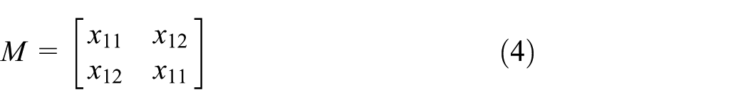


where R is half of the width of the tracked robot and r is the radius of the wheels which drive the tracks. M is the inertia matrix symmetric and positive defined by the physical parameters of the tracked robot,

Schematic model of a tracked mobile robot, where x, y are the coordinates of
Neural networks
Artificial neural networks also known as neural networks are massively parallel distributed processors built of a massive interconnection of simple computing units called neurons; they are designed to model the way in which the brain performs a task or a function; 27 in other words, artificial neural networks are simplified models of the biological neural networks which we can implement in software or hardware.27–29 Neural network computing power comes from its massive interconnection and its ability to learn and generalize. 27
According to their architecture, neural networks can be classified as follows:10,27,28
Static neural networks. These kinds of neural networks are capable of approximating any function using a static mapping.
Dynamic neural networks. These types of neural networks have feedback connections which give them higher capability than static neural networks. Due to their feedback connection, dynamic neural networks are capable of capturing the dynamic response of a system.
Neural networks are usually implemented using electronic components or simulated in software. 27
RHONN
RHONNs are dynamic neural networks which are capable of capturing the dynamic response of complex non-linear systems10,30 and also systems with time delay
15
due to characteristics such as a flexible model that allows us to incorporate a priori information about the system to be identified, approximation capabilities, robustness against noise, on-line training and their dynamical behaviour that is the result of their recurrent connections that improve their learning capabilities and performance.10,30 RHONNs are the result of including high-order interactions represented by triplets (
The RHONN model used in this work is the series–parallel model model, 10 which is defined as

with


where n is the state dimension,
Neural network training
Neural network training is a process in which the neural network learns a task; this training can be on-line or off-line.27,28 The most common training algorithms for static neural networks and dynamic neural networks are backpropagation and backpropagation through time learning, respectively.27,28,31
Kalman filter
It estimates the state of a linear system with additive state and output white noise using a recursive solution in which each update of the state is estimated from the previous estimated state and the new input data.10,31
Kalman filter training
Kalman filter training for neural networks offers advantages such as reduction in the epoch number and number of required neurons, on-line and off-line training implementation, improvement in learning convergence and also they are more computationally efficient compared to the most used backpropagation methods.10,31 Moreover, they have proven to be reliable and practical.10,27
The training goal is to find the optimal weight vector which minimizes the prediction error. Due to the fact that the neural network mapping is non-linear, EKF is required.
EKF-based training algorithm
It estimates the neural network weights which become the state, and the error between the measured output of the plant and the output of the neural network is considered as additive white noise.10,31
The EKF-based training algorithm 10 for RHONN series–parallel model (10) is equation (14)

with


where
Neural identification
Neural identification consists in selecting an appropriated neural network model and adjusting its weights according to an adaptation law, so that the neural network approximates the real system response for the same input. 33 Now let us consider the following non-linear discrete time-delay multiple input, multiple output (MIMO) system described by

where
We use a model with time delay because the wireless communication with the tracked robots could induce some delays and we can modify the series–parallel model (10) to accept a state vector of a plan with time delays; 15 therefore, we get the following model

This model is semi-globally uniformly ultimately bounded and the proof can be found in Alanis et al. 15 The RHONN series–parallel model (18) is selected to identify model (17), and the EKF-based algorithm (14) is used as the adaptation law.
Inverse optimal control
Consider the following affine discrete non-linear system (19)

where
For the inverse optimal control, a Lyapunov control function is design to satisfy the passivity condition which states that a passive system can be stabilized by making a negative feedback from the output.
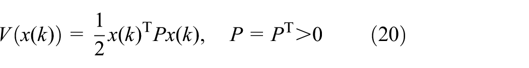
Instead of solving the associated HJB equation, the inverse optimal control synthesis is based on the knowledge of
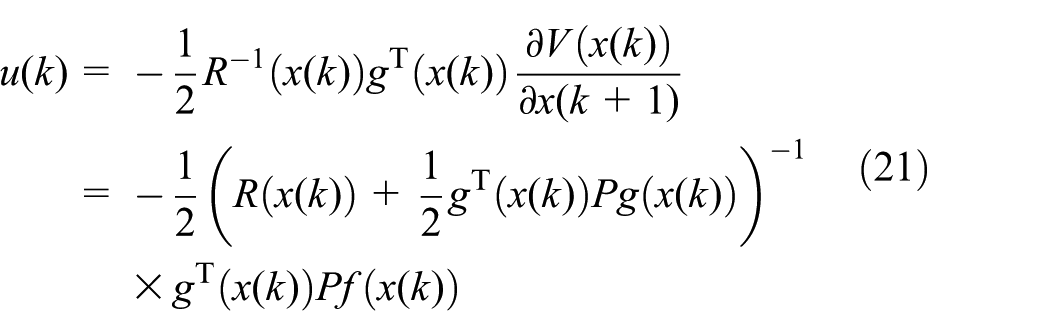
where

with


In Sanchez and Ornelas-Tellez, 17 it is demonstrated that control law (21) is globally asymptotically stable. Moreover, equation (21) is inverse optimal in the sense that it minimizes a cost functional. 17
Application to a tracked mobile robot
Figure 2 shows the closed loop for neural identifier – inverse optimal control scheme.

Control scheme.
Neural identification of a tracked robot
The discrete-time RHONN identifier (28) is proposed to get a valid mathematical model for tracked mobile robots

where
RHONN identifier (28) is adapted on-line using the EKF-based training algorithm (14). All the neural network states and weights are initialized in a random way.
Inverse optimal control of a tracked robot
The control objective is the design of a control law u to track the desired trajectory generated by the following reference robot

where xr, yr and
The design of a controller based on model (1) requires the exact knowledge of the plant parameters and disturbances which can vary with time; since in practice getting this model is not a trivial task, the identified model (28) is used as a valid model for the tracked robots, and therefore, the identified model (28) is used to design the controller for solving the trajectory tracking problem.
Systems (1) and (29) are discretized based on the Euler methodology. System (1) is rewritten in the block structure form (30) to simplify the controller synthesis

where
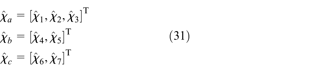

with


In this way, the control objective is to force xa to track the reference signal

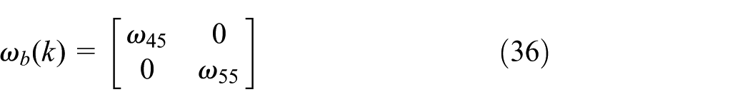
Therefore, the reference signal for the control law

with

where
Results
This section presents the simulation and real-time results. The simulations of model (1), RHONN identifier (28) and control (40) were implemented in MATLAB and Simulink® (MathWorks, Inc.) software. On the other hand, in the real-time tests, the block that represents the model of the robot was removed and replaced with a block where the communication with HD2 was implemented.
In this way, it was demonstrated that the same RHONN identifier is capable of identifying both the models, the one used for simulation and the one for HD2. Also, due to the fact that the control was designed using the model of RHONN identifier, it is valid for both simulation and real-time tests. The parameters for RHONN identifier for all tests are shown in Table 1.
EKF-based training algorithm parameters.

Moreover, the following weights are fixed:
Simulation
Simulation test
The parameters for the test are set as follows


where T is the sample time.
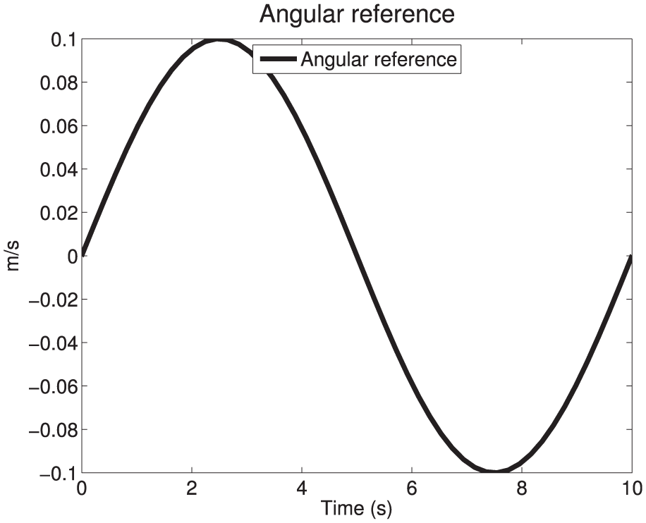
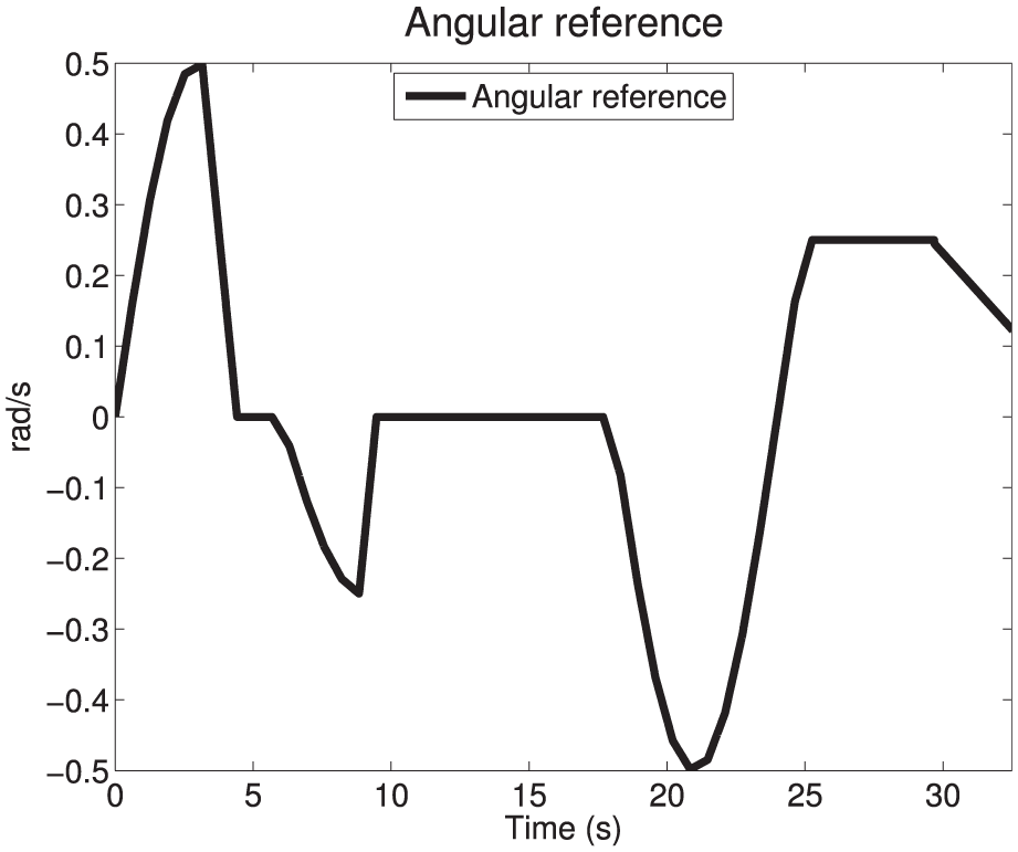
Figures 3 and 4 show the references for linear and angular velocities, respectively.

Linear velocity reference for simulation test.

Angular velocity reference for simulation test.
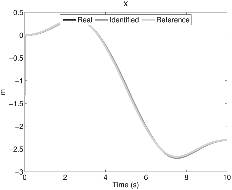
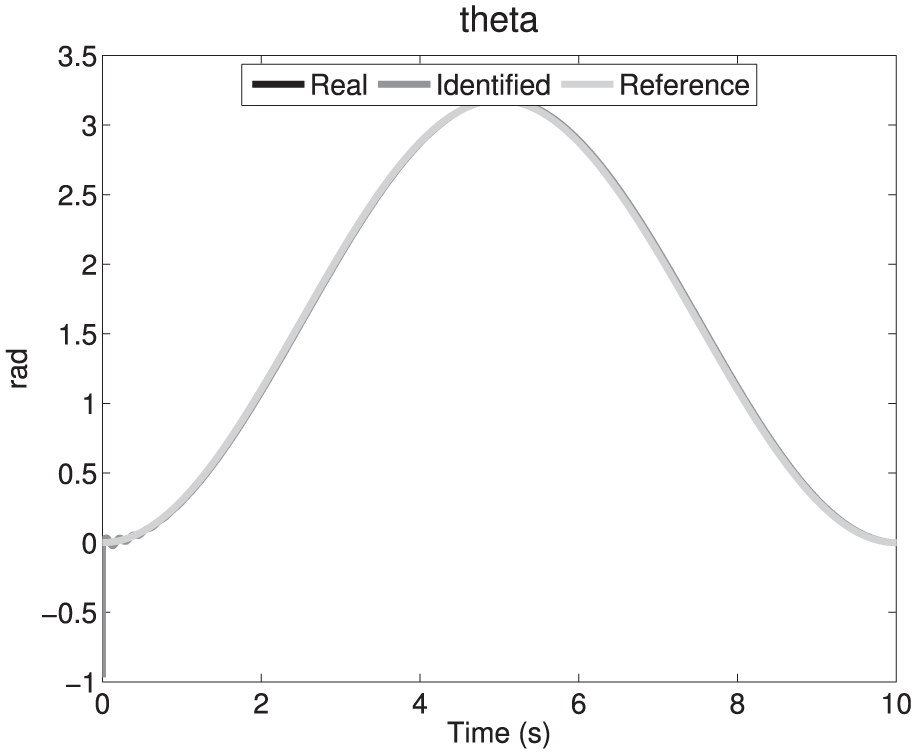
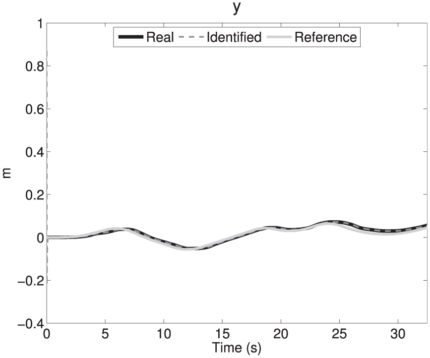
Figures 5–7 show the references, real and identified signals of x, y and

Real, identified and reference signals of x of simulation test.

Real, identified and reference signals of y of simulation test.
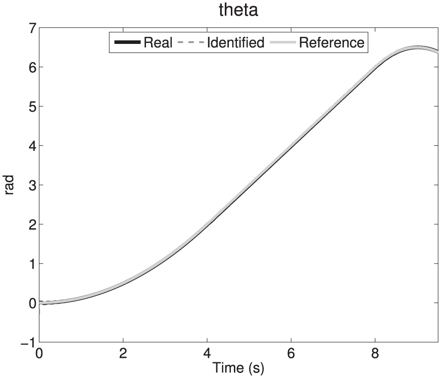
Real, identified and reference signals of
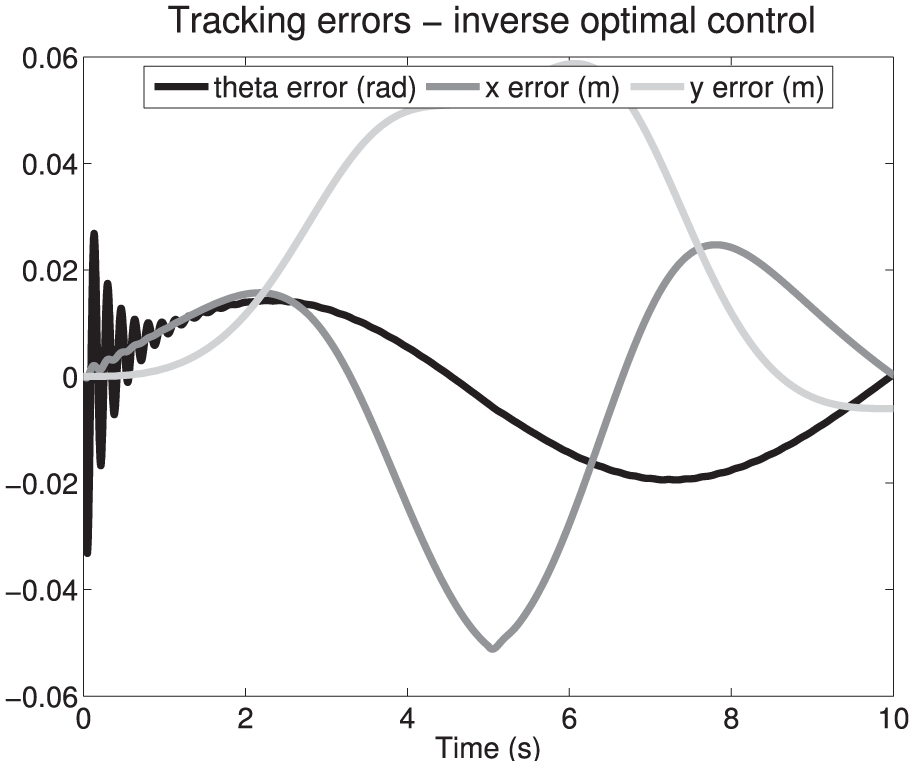
The errors of the simulation test are shown in Figure 8 and Table 2. Figure 8 shows the errors of reference versus simulated real signals; a comparison between reference signals and identified signals is omitted because the error between the real and identified signal is so small that a second figure showing the reference versus identified signal would look just like Figure 8.
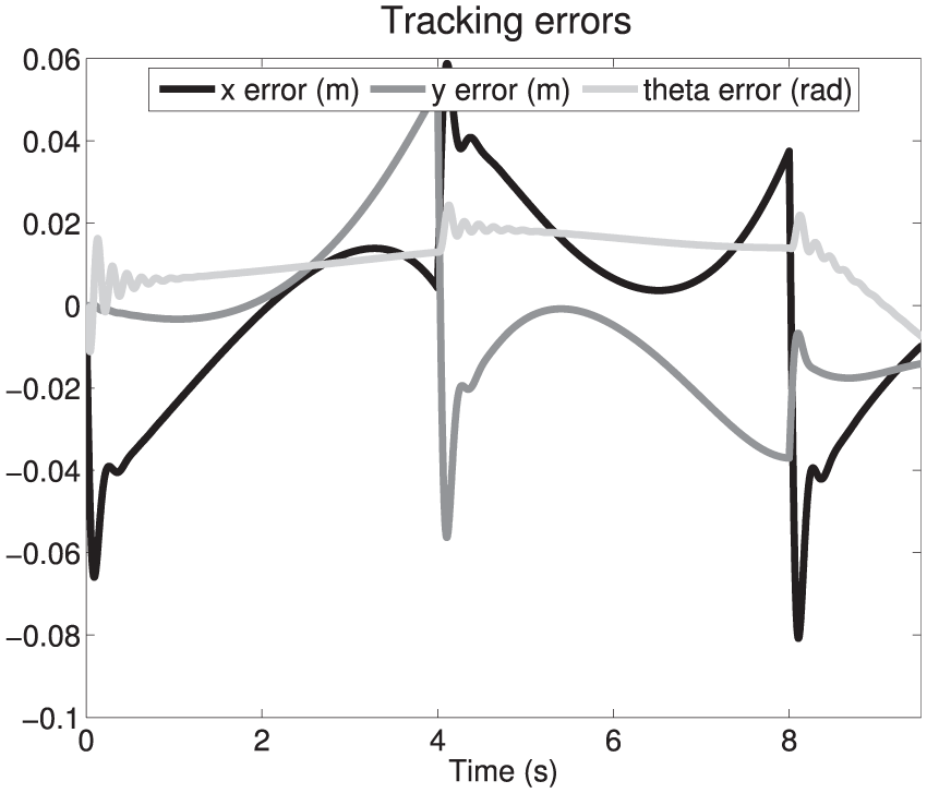
Tracking errors of simulation test.
RMSE of simulation test tracking errors of x, y and

RMSE: root mean square error.
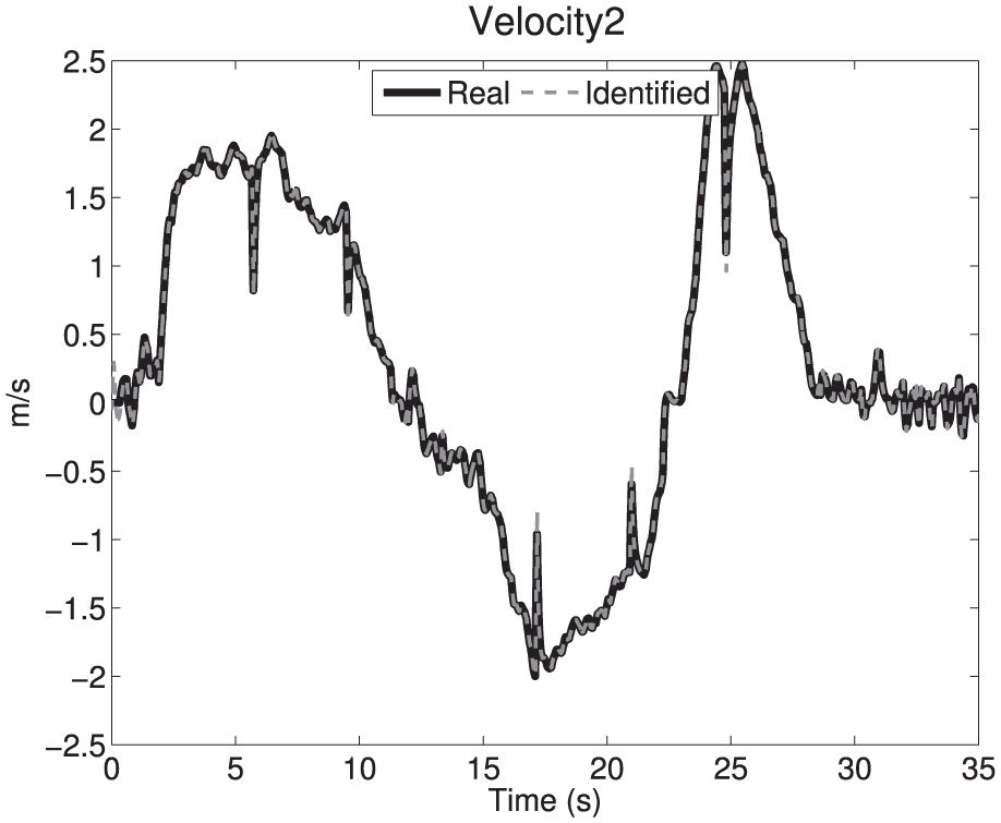
Figures 9 and 10 show the velocities v1 and v2, respectively.

Real and identified signals of v1 of simulation test.

Real and identified signals of v2 of simulation test.
Figures 11 and 12 show currents i1 and i2, respectively.

Real and identified signals of i1 of simulation test.

Real and identified signals of i2 of simulation test.
Figures 13 and 14 show control signals u1 and u2, respectively.

Control signal u1 of simulation test.

Control signal u2 of simulation test.
Table 3 shows the root mean square error (RMSE) of the real versus identified signals.
RMSE of simulated real versus identified state variables of simulation test.
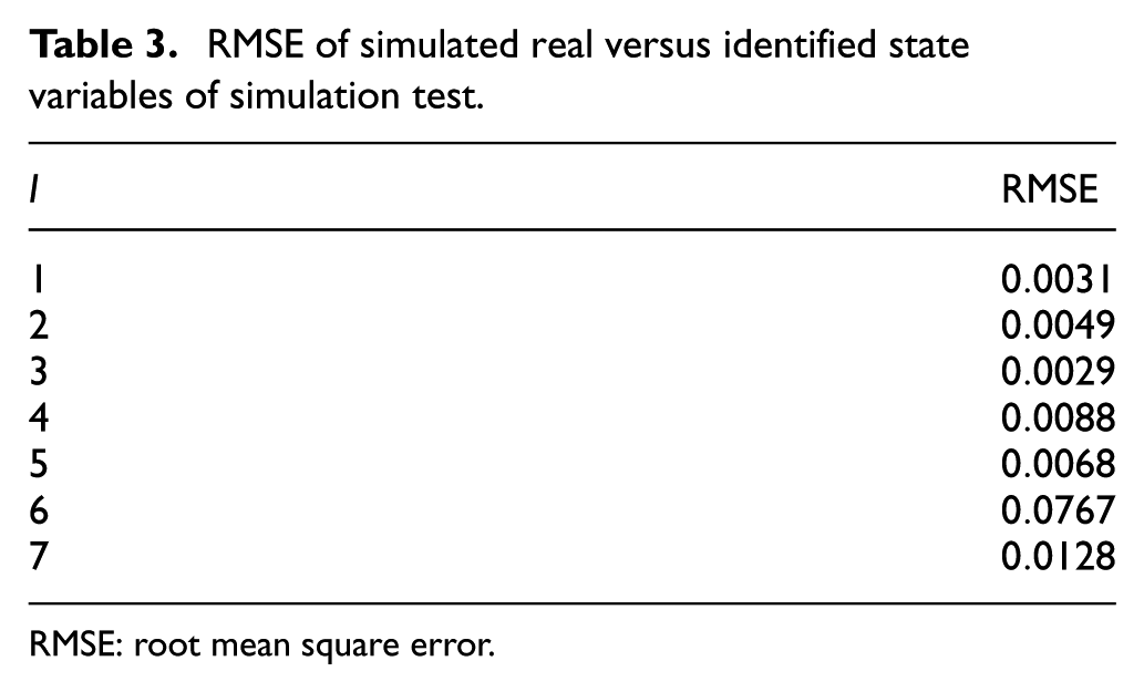
RMSE: root mean square error.
Performance comparison
The following simulation results compare the proposed neural identifier – inverse optimal control scheme – and the super twisting control proposed in Lopez-Franco et al., 25 which is a discrete-time control algorithm for nonholonomic wheeled mobile robots, without the previous knowledge of the plant model or its parameters. The super twisting control proposed in Lopez-Franco et al. 25 was adapted from the three-state model presented in Lopez-Franco et al. 25 to our seven-state model. For comparison, we use the same references shown in Figures 15 and 16.

Linear velocity reference for the performance comparison test.
Angular velocity reference for the performance comparison test.
The tracking performance for the neural identifier – inverse optimal control – is shown in Figures 17–19, for x, y and
Real, identified and reference signals of x with neural identifier: inverse optimal control.

Real, identified and reference signals of y with neural identifier: inverse optimal control.
Real, identified and reference signals of

Real and reference signals of x with super twisting.
Real and reference signals of y with super twisting.
Real and reference signals of
For more details, Figures 23 and 24 show the errors and Table 4 shows the RMSEs of the tests.
Tracking errors with neural identifier: inverse optimal control.

Tracking errors with super twisting.
RMSE of simulation comparison test tracking errors of x, y and

RMSE: root mean square error.
Figures 15 to 24 and Table 4 show that a better performance is found in the neural identifier – inverse optimal control scheme compare to the super twisting in states x and, especially, in
Real-time
Figure 25 shows the HD2 Treaded ATR Tank Robot Platform with an added wireless router.

HD2® Treaded ATR Tank Robot Platform.
Figure 26 shows the HD2 Treaded ATR Tank Robot Platform inside where the modification of the platform can be seen. Basically, the modification is the replacement of the original board with a system based on Arduino® (Arduino LLC) and added current sensors; Figure 26 also shows the original batteries and motors.

HD2® Treaded ATR Tank Robot inner components.
Real-time test 1
The parameters for the real-time test are set as follows


Figures 27 and 28 show the references for linear and angular velocities, respectively.

Linear velocity reference for real-time test 1.

Angular velocity reference for real-time test 1.
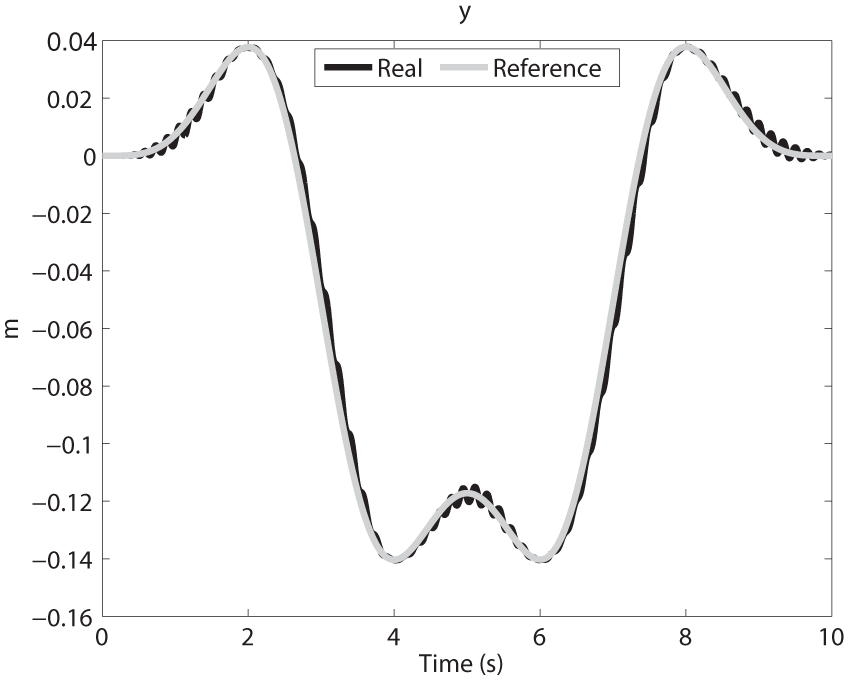
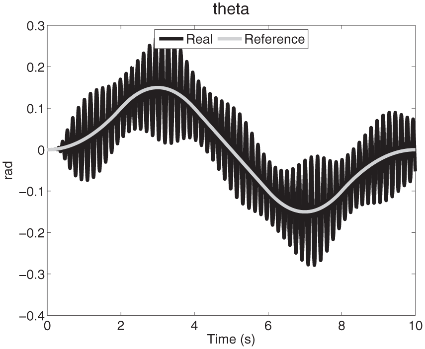
Figures 29–31 show the references, real and identified signals of x, y and

Real, identified and reference signals of x of real-time test 1.

Real, identified and reference signals of y of real-time test 1.

Real, identified and reference signals of
In contrast to the simulation results, the presented real-time tracking results of Figures 29–31 cannot achieve a perfect tracking mainly to the following reason:
WiFi communication and packet loss;
Actuators’ saturation;
Noise and precision of the sensors;
Unmodelled dynamics.
However, they have the same dynamic and small errors shown in Figure 32 and Table 5; also, it is important to mention that this is accomplished without the knowledge of our modified tracked robot model and parameters.

Tracking errors of real-time test 1.
RMSE of real-time test 1 tracking errors of x, y and

RMSE: root mean square error.
Figures 33 and 34 show velocities v1 and v2, respectively.

Real and identified signals of
Real and identified signals of
Figures 35 and 36 show currents i1 and i2, respectively.

Real and identified signals of

Real and identified signals of
Figures 37 and 38 show control signals u1 and u2, respectively.

Control signal

Control signal
Table 6 shows the RMSE of the real versus identified signals.
RMSE of real versus identified states of real-time test 1.

RMSE: root mean square error.
Real-time test 2
The parameters for this test are the same as the previous test. Figures 39 and 40 show the references for linear and angular velocities, respectively.

Linear velocity reference for real-time test 2.
Angular velocity reference for real-time test 2.
Figures 41–43 show the references, real and identified signals of x, y and

Real, identified and reference signals of x of real-time test 2.
Real, identified and reference signals of y of real-time test 2.

Real, identified and reference signals of
The errors of real-time test 2 are shown in Figure 44 and Table 7.

Tracking errors of real-time test 2.
RMSE of real-time test 2 tracking errors of x, y and

RMSE: root mean square error.
Figures 45 and 46 show velocities v1 and v2, respectively.

Real and identified signals of
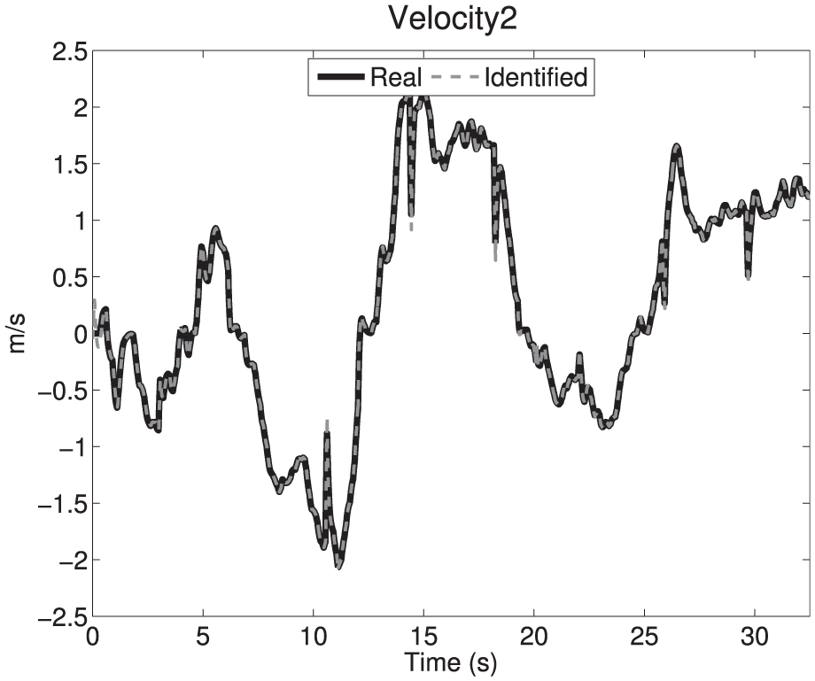
Real and identified signals of
Figures 47 and 48 show currents i1 and i2, respectively.
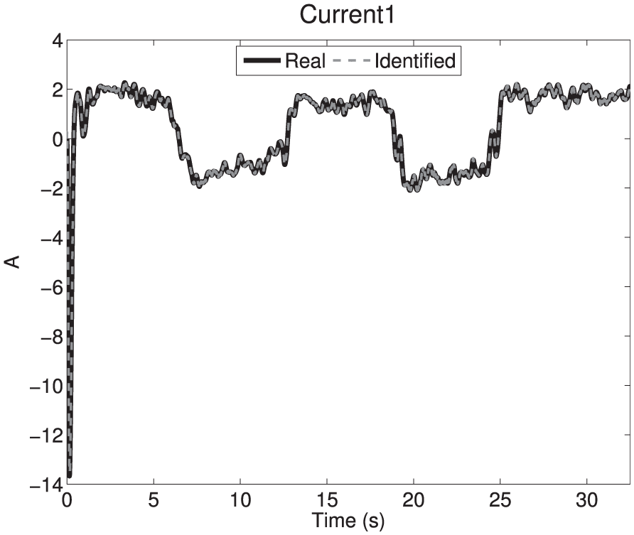
Real and identified signals of

Real and identified signals of
Figures 49 and 50 show control signals u1 and u2, respectively.

Control signal

Control signal
Table 8 shows the RMSE of the real versus identified signals.
RMSE of real versus identified states of real-time test 2.
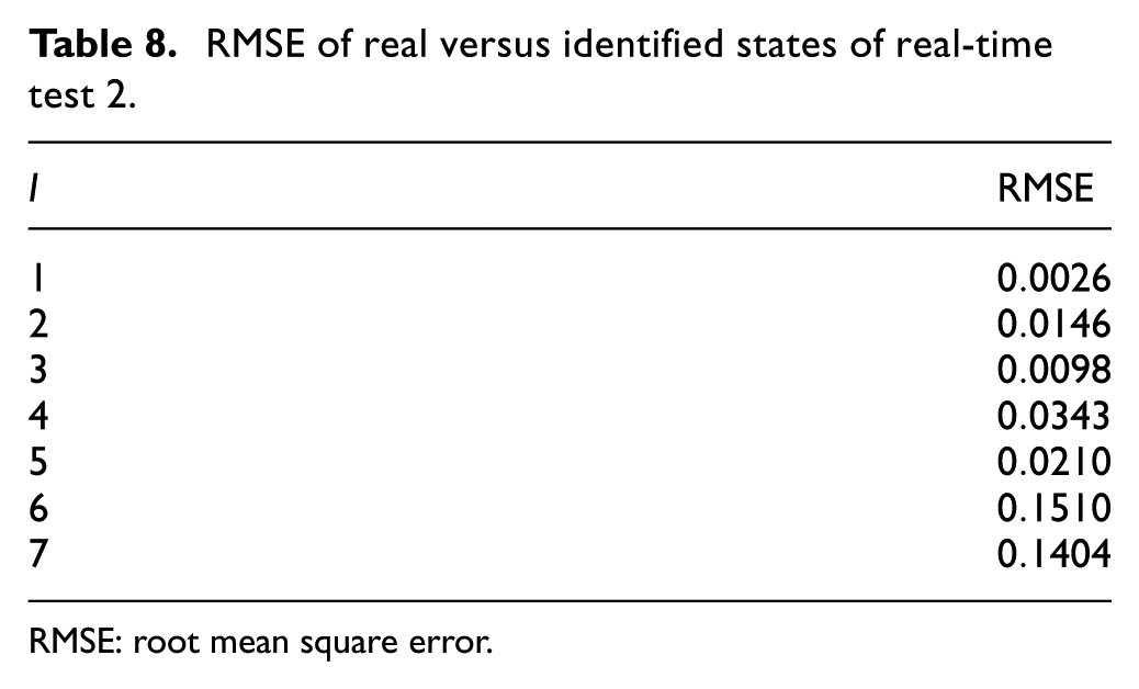
RMSE: root mean square error.
Conclusion
This work uses an RHONN identifier trained with an EKF-based algorithm to get the model of a simulated plant to identify and the model of an actual tracked robot. Through the results, it can be seen that the same neural identifier was capable of identifying both simulated and real models, with sample times equal to 0.001 and 0.003 s, respectively.
It is important to say that the knowledge about the model parameters of our modified HD2 was not available. Moreover, for simulation even if the parameters were available, they were not used for the design of the identifier.
On the other hand, the inverse optimal control which was designed using the identified model shows good results for simulation and real-time tests. This can be appreciated in the result graphs which compare the references against the real signals of the robot.
Footnotes
Academic Editor: Jianyong Yao
Declaration of conflicting interests
The author(s) declared no potential conflicts of interest with respect to the research, authorship, and/or publication of this article.
Funding
The author(s) disclosed receipt of the following financial support for the research, authorship, and/or publication of this article: The authors thank the support of CONACYT Mexico, through projects CB256769 and CB258068 (‘Project supported by Fondo Sectorial de Investigación para la Educación’).