Sage Journals: Discover world-class research

Abstract

The joint robots are used in kinds of production processes. A fast time work load identification is the premise to ensure the safe operation of robots. However, in some special application scenarios, the work load can not be measured directly, which is often identified indirectly by dynamic methods. Because of the obvious nonlinearity and the uncertainty of model parameters, the accuracy and efficiency of load identification are not enough. Therefore, based on Fourier neural network, this paper proposes an improved model to realize load identification, in order to improve the prediction accuracy and timeliness of system load parameters. Compared with the dynamic model solution method, the proposed method has higher accuracy and faster calculation speed. It only needs to learn several alternate sample sets in the prediction range, and any results in the prediction range can be accurately identified with good generalization ability. The sensitive parameters of the network are also analyzed, and the performance is compared with that of mature neural network algorithm. In this method, two neural network models are combined to effectively identify different feature sets in high-dimensional data, so as to realize efficient load parameter identification and provide reference for parameter identification of complex nonlinear systems.

Keywords

industrial robot Fourier neural network dynamics real-time load identification

Introduction

Motivations

Real-time load identification or monitoring of industrial robots is an important prerequisite for ensuring smooth operation, state analysis, and precise control of the system.¹ The working load has correlation with the service life and working intensity of the robot.^2,3 However, in some special scenes, such as vacuum, high humidity, strong magnetism, and large vibration, the torque sensors are prone to data distortion or even damage. Thus the load identification must be carried out by indirect methods such as dynamic analysis and deep learning.⁴ Because the robot has the characteristics of high-dimensional nonlinearity, its dynamic parameters will change with the running time, which will affect its load identified accuracy. Therefore, the deep learning algorithm is generally applied for improving its identified accuracy.^5,6

For a joint type robot with strong nonlinearity, the robot’s dynamic parameters maybe change under different tasks. If the load identification and control parameters are not adjusted to the change, it will cause unexpected vibration or abnormal wear.⁷ In identification of the load, a comparatively complete dynamic model is generally applied for evaluating working load under the real-time testing. However, some parameters of the dynamic model, such as frictional coefficient, damping coefficient, may change over the running time and are difficult to measure.⁸ The analysis results may be affected by the inaccuracy of input parameters.

In addition, due to the existence of nonlinearity, the calculation amount is very large when solving with the dynamic model. Therefore the numerical methods are used for analysis. But the efficiency of the numerical method is low under the condition of large excitation variation and complex working conditions.¹ Consider that the deep learning can simulate the complex changes in nonlinear systems, which has been widely used in many fields, such as medical analysis,^9,10 image recognition,¹¹ structural analysis,¹² target optimization,¹³ and so on. Thus the purpose of this paper is to develop a real-time load identification method of multi-degree of freedom robot based on an improved Fourier neural network.

Literature reviews and objectives

In order to meet the high precision and timeliness of industrial robot load identified, the effective application and accurate analysis of small sample data are the key points of research. Aiming at the problems of redundancy of a large amount of data and low diagnosis accuracy in fault diagnosis methods, Pan et al.¹⁴ proposed a weighted training model of convolution neural network. And the fault diagnosis rate is improved by 28.6%. Aiming at the problem of small and unbalanced data in impact damage experiment, combined with classifier segmentation technology, Doan et al.¹⁵ proposed an automatic classification model with high stability. Zhang et al.⁷ established a linear identification model of Lagrange dynamics to effectively identify the load and parameters of robot. The dynamic solution method can meet certain precision requirements, but its calculation process is complicated and the computational time is long.

The joint type robot belongs to a kind of highly coupled nonlinear system, and the nonlinear factors are difficult to consider. The parameters are uncertain, and the dynamic differential equations of the system are complex and the solution time is long. Therefore, how to use sample data quickly and accurately to learn or simulate the solution process of differential equations has become a new research hotspot. Raissi et al.⁶ put forward Physical Information Neural Network algorithm (PINN) with data physical mechanism learning process. The difference before and after iteration of physical equations were added to the loss function of neural network for training by PINN, so that the training results have physical laws and achieve efficient learning effect. Raissi et al.¹⁶ extended the PINN algorithm and applied it to implicit hydrodynamics calculation, so that the algorithm is not limited to specific boundary and initial conditions. Zhu et al.¹⁷ integrated the governing equations of the physical model into the loss function to realize the optimization of the algorithm. Bar-Sinai et al.¹⁸ proposed a method based on machine learning and automatic discretization of continuous physical equations.

Li et al.¹⁹ proposed a Fourier Neural Operator (FNO), which extends neural networks to learn mappings in function spaces to solve partial differential equations (PDEs). By directly parameterizing the integral kernel in the Fourier space, they constructed an efficient architecture successfully applied to solving the Burgers equation, Darcy flow equation, and Navier-Stokes equation. Experimental results demonstrated that FNO is three orders of magnitude faster than traditional PDE solvers and achieves higher accuracy at fixed resolutions. The purpose of FNO is to replace complex mathematical solvers, with its training data derived from dynamic equations that represent the general, fundamental, and relatively simplified dynamics model information during robot operation. By leveraging the frequency domain characteristics of Fourier transforms, FNO’s advantages include reduced computational complexity, improved computational efficiency, and decreased reliance on grid refinement and precise data. These features make it particularly suitable for addressing complex nonlinear problems, such as those encountered in robotics.

In addition, Lample and Charton²⁰ built a neural network model for solving analytical solutions of differential equations based on seq2seq model of natural language processing. And the results were equivalent to those of commercial software, but the solving process was complicated. Neural networks can be applied in various scenarios, such as medical diagnosis,²¹ perception and decision-making,²² and intelligent control.²³ These advanced neural network methods solve the problems of multimodal time series classification, small-shot learning, and robot control to a certain extent. It can provide innovative ideas for robot control. In order to achieve the result when it was impossible to solve the strong solution of differential equation, Zang et al.²⁴ put forward a weak adversarial network (WAN) model based on the weak solution of partial differential equation. A loss function was constructed to solve the solution of differential equation through the generating countermeasure network (GAN). If the Fourier transform is integrated into neural network model, the computational complexity of the model can be effectively reduced. The physical laws in data can be effectively captured through the Fourier transform, which has great advantages for solving partial differential equations. Mathieu et al.²⁵ calculated convolution as dot-by-dot product in Fourier domain, and reused the same transform feature map many times to accelerate the training of neural network. Li et al.¹⁹ put forward the neural network with invariant grid into solving the partial differential equations. The computational efficiency was greatly improved. Vahid et al.²⁶ extended the butterfly transform in the traditional fast Fourier transform and applied it to the architecture design of convolution neural network. The results showed that the computational complexity of the network layer after butterfly transform is reduced from o(n²) to o(nlogn), and experiments showed that the proposed method can also improve the accuracy.

For strong nonlinear systems with a lot of computation time, it is still difficult to meet the requirements of timeliness and high accuracy only by using mathematical methods for parameter identification and state recognition. Therefore, this paper proposes an improved Fourier neural network model to replace the dynamics model for load identification, so as to improve the prediction accuracy and timeliness of system parameters.

The organization of this paper is as follow. Firstly, the improved Fourier neutral network is established for load identification in Section “Improved Fourier neural network.” Then the UR5 of multi-degree of freedom robot is set as the object of study, and the measured excitation and the process of data acquisition are given in Section “Test platform and data acquisition.” In Section “Load identification and analysis based on dynamic model,” the dynamic modeling for the multi-degree of freedom robot is established, and the load identified by dynamic method is given and analyzed. In Section “Load identification and analysis using improved Fourier neural network,” the load identification by the proposed method is given, the influence factors are analyzed, and a strategy for improving the load identified accuracy is proposed. Conclusions are drawn in Section “Conclusion.”

Improved Fourier neural network

Fourier neural network

The Fourier neural network (FNO) is a network architecture with convolution structure and Fourier transform. Fourier transform can transform data into frequency domain and retain important parts of information. The convolution structure can reduce the memory occupied by deep network and extract important features from source information. The gradient descent method is used to minimize the loss function and update the network parameters layer by layer, and iterative training is used to improve the prediction accuracy of the network.

Network architecture

The structure of Fourier neural network is shown in Figure 1.

Figure 1.

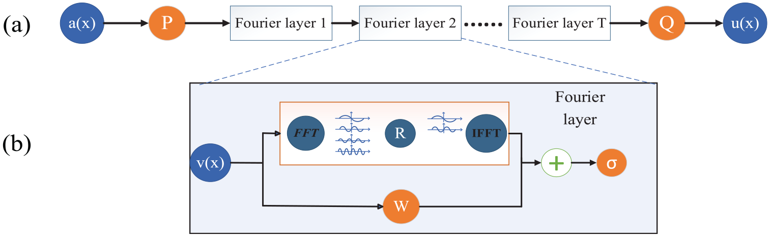
The architecture diagram of Fourier Neural Network (FNO): (a) is Fourier neural networks and (b) is Fourier layer detail.

In Figure 1, the FNO complete architecture of process (a) is described as follows. Firstly, the input data is set as a(x). The data is upgraded to a higher dimensional channel space through neural network P. The Fourier layer includes T-layer integral operator and an activation function Q. The target dimension is returned by neural network Q. At last, the value u is output.

The explanation of Fourier layer is given here. Firstly, the input data is set as v(x). In the upper half region, the Fourier transform FFT is applied for converting the data into frequency domain. The low frequency signal is linearly transformed, and the higher frequency signal is filtered out. Then the inverse Fourier transform IFFT is applied for converting the data into time domain. In the lower half region, a local linear transform W is applied for extracting the feature signal.

Operation principle

FNO iterative algorithm:

\begin{matrix} v_{1} (x) = P (a (x)) \end{matrix}

(1)

\begin{matrix} v_{t + 1} (x) = σ (W v_{t} (x) + (K (a; ϕ) v_{t}) (x)) \end{matrix}

(2)

\begin{matrix} u_{x} = Q (v_{T} (x)) \end{matrix}

(3)

In the above formula: P is a matrix that projects low dimensions to high dimensions, and Q is a matrix that projects high-dimensional vectors to low dimensions, all of which are projection operators, in order to increase the characteristic dimensions of neural networks;

Definition of Fourier integral operator:

(K (a; ϕ) v_{t}) (x) = \int K (x, y, a (x), a (y)) v (y) dy

(4)

The expression of Fourier transform is as follows:

\begin{matrix} {(Ff)}_{j} (k) = \int f_{j} (x) e^{- 2 i π (x, k)} dx \end{matrix}

(5)

\begin{matrix} {(F^{- 1} f)}_{j} (x) = \int f_{j} (k) e^{2 i π (x, k)} dk \end{matrix}

(6)

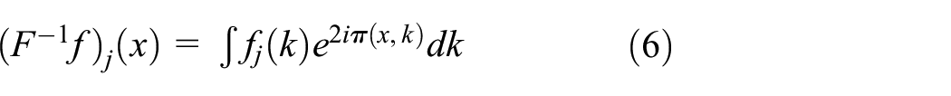
From equations (5) and (6), we can deduce that the integral operator is:

\begin{matrix} (K (a; \emptyset) v_{t}) (x) = F^{- 1} (F (k_{\emptyset}) \cdot F (v_{t})) (x) \end{matrix}

(7)

In this way, the Fourier integral operator can be written as:

(K (\emptyset) v_{t}) (x) = F^{- 1} (R_{\emptyset} \cdot (F v_{t})) (x)

(8)

Therefore, the Fourier neural operator is proposed to solve the integral term in operator learning, and then combined with the above iterative relationship, the mathematical principle of the model can be expressed.

\begin{matrix} v_{t + 1} (x) = σ (W v_{t} (x) + (K (a; ϕ) v_{t}) (x)) \end{matrix}

(9)

Improved Fourier neural network model

The original data dimension of the load identification experiment is that there are nine groups of different load values, and each group of load experiments produces 120,000 × 54 data points. Based on Anaconda 4.8. 3 platform, using Python 3.9, Pytorch, and other library functions, this paper explores the improvement of Fourier neural network load forecasting ability. Among them, 80% are training data and 20% are test data, which are labeled with actual load value, so as to explore the load prediction effect of machine learning. $[9, 50 * 2400, 54]$

Improve the network architecture

In Figure 2, the FNO_FFNN complete architecture of process (a) is described as follows. Firstly, the input data is set as a(x). The data is upgraded to a higher dimensional channel space through neural network P. The Fourier layer includes N-layer integral operator, M-layer feedforward neural network (FFNN_net) linear layer, and an activation function Q. Then the information of FNO and FFNN is fused. The target dimension is returned by neural network Q. At last, the value u is output.

Figure 2.

The modified architecture diagram of Fourier Neural Network (FNO_FFNN): (a) FNO_FFN overall structure and (b) FNO_FFN layer detail.

The explanation of Fourier layer is given here. Firstly, the input data is set as v(x). In the upper half region, the Fourier transform FFT is applied for converting the data into frequency domain, and the linear transform R is used for intercepting the frequency general medium and low frequency information. Then the inverse Fourier transform IFFT is applied for converting the data into time domain. In the lower half region, a local linear transform W is applied for extracting the feature signal.

Loss function

Mean square error (MSE) and least square error (LPLoss) are selected as the loss and evaluation functions of this model. The function curve of MSE is smooth, continuous, and can be derived everywhere, so it is easy to use gradient descent algorithm, and it is a common loss function. Moreover, with the decrease of error, the gradient also decreases, which is beneficial to convergence. Even with a fixed learning rate, it can converge to the minimum value quickly. The formula is as follows:

MSE = \frac{1}{n} \sum_{i = 1}^{n} {(f (x) - y)}^{2}

(10)

where $f (x)$ is the output value of neural network model, y is the actual label, and n is the number of samples.

LPLOSS is suitable for many types of neural network models and tasks, including regression, classification, etc. Different norms can be selected according to needs, and it is suitable for model training in different scenarios. Through the calculation of relative errors, the symbolic information of errors is retained, so that positive and negative errors can cancel each other and reflect the model performance more accurately.

LP = \frac{1}{n} \sum_{i = 1}^{n} \sqrt[p]{{(\frac{f (x) - y}{y})}^{p}}

(11)

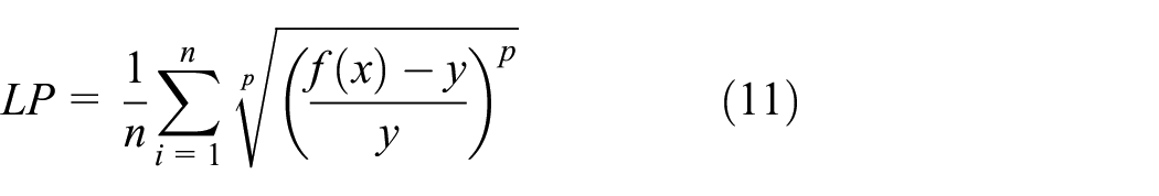
where $f (x)$ is the output value of neural network model, y is the actual label, n represents the number of samples, and p represents the norm. Here the value of p is selected as two in this paper.

Model parameters

Build a training model, and complete the construction of neural network according to the size of source data. See Table 1 for specific model parameters.

Table 1.

The model parameters of modified Fourier neural network model.

Network layer	Output dimension	Parametric quantity
Linear-1	[1, 54, 64]	912
SpectralConv1d-2	[1, 64, 54]	0
Conv1d-3	[1, 64, 54]	4160
SpectralConv1d-4	[1, 64, 54]	0
Conv1d-5	[1, 64, 54]	4160
SpectralConv1d-6	[1, 64, 54]	0
Conv1d-7	[1, 64, 54]	4160
SpectralConv1d-8	[1, 64, 54]	0
Conv1d-9	[1, 64, 54]	4160
Linear-10	[−1, 64, 128]	7040
Linear-11	[−1, 64, 64]	8256
Linear-12	[−1, 64, 128]	8320
Linear-13	[1, 64, 54]	6966
Linear-14	[−1, 540, 10]	650
Flatten-15	[−1, 540]	0
Linear-16	[−1, 1]	541

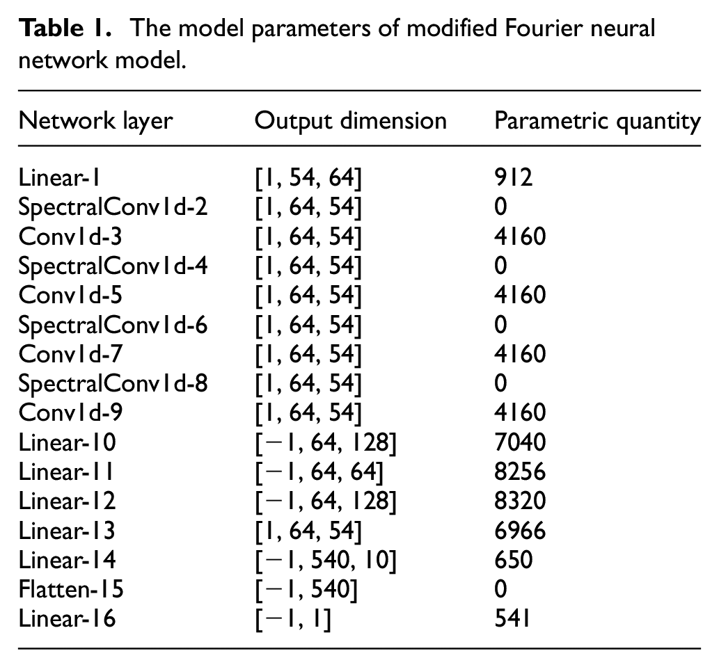
The total parameters of the improved Fourier neural network load forecasting model (FNO_FFNN) are 48,605. The training parameters are set with reference to the number of original data and the size of dimensions. After many adjustments, the number of layers and the parameters of each hidden layer of the model are determined. In order to ensure the integrity of data, the convolution layer is set with padding as same, activation function as gelu function, optimizer as Adam, loss function as MSE and LPLoss, and evaluation function as LPLoss.

Test platform and data acquisition

Load identification experiment

In this paper, the six-degree-of-freedom robot UR5 is taken as the research object, and the trajectory excitation of typical finite Fourier series excitation is taken as the trajectory of UR5 robot. The structure and trajectory design of UR5 robot are shown in Figure 3. The system can collect the motion parameters and current values of each robot joint, and no torque sensor is installed at each joint.

Figure 3.

The design motion path of UR5 Robot: (a) structural diagram of UR5 Robot, (b) robot joint coordinates, and (c) the exception motion of Joint 2.

Data acquisition and processing

The UR5 robot can output nine process quantities of each joint which are actual position, actual speed, actual current, control current, target position, target speed, target acceleration, and target torque. When the load changes, the movement is completed according to the excitation trajectory. In order to reduce contingency, each load repeated 50 qtimes, and a total of 450 groups of experimental data are used as original data. The characteristic signals such as position, speed, and current of the robot are collected at the frequency of 125 Hz, and some source data are shown in Figure 4.

Figure 4.

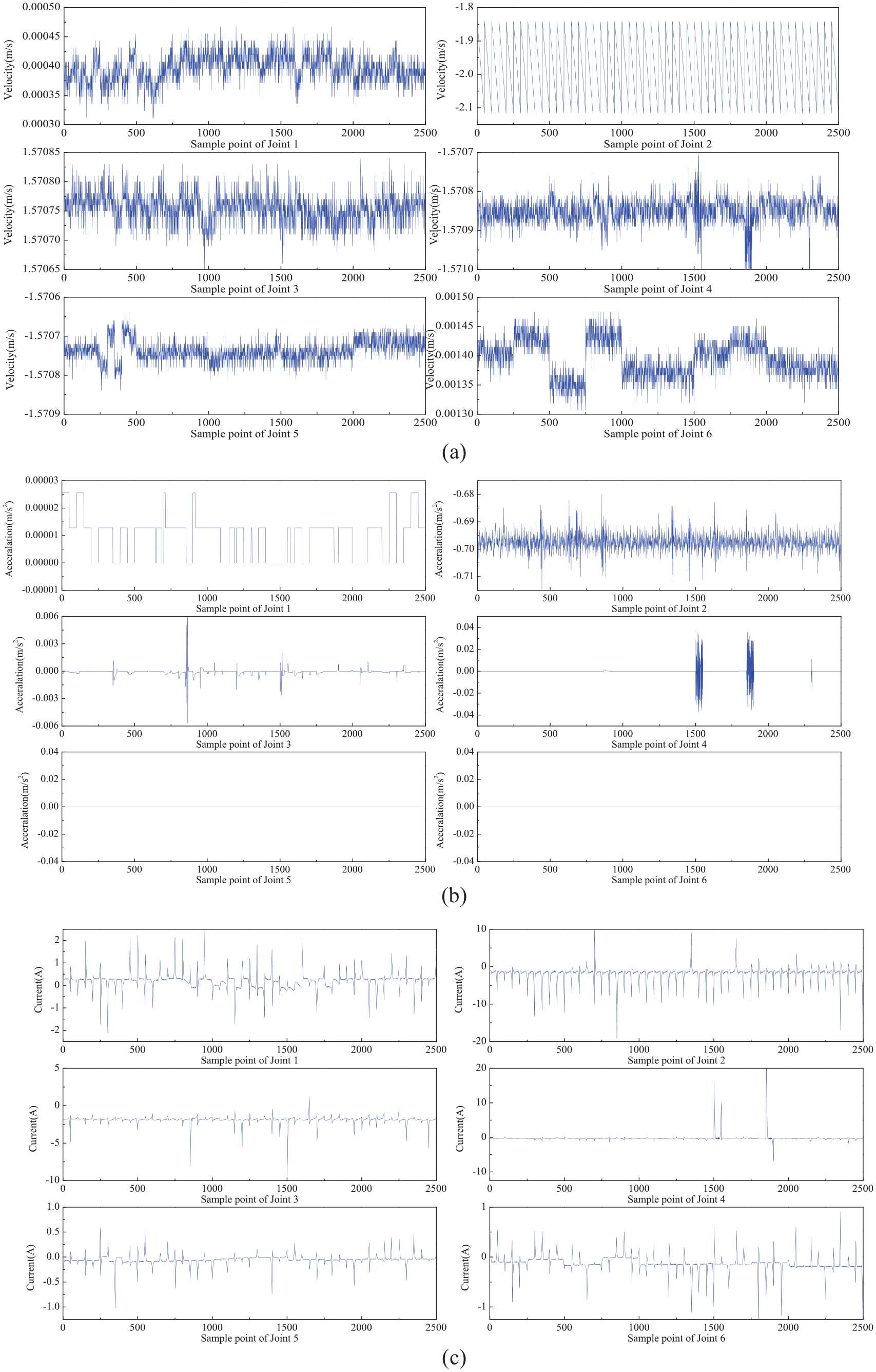
The part of the collecting source data: (a) actual velocity of source data, (b) target acceleration of source data, and (c) actual current of source data.

Figure 4(a) shows the actual velocity of joint 1, joint 3, and joint 5. Figure 4(b) shows the target acceleration of joint 2, joint 4, and joint 6. Figure 4(c) shows the actual current of joint 1, joint 3, and joint 5. It can be seen that there are great differences in joint data, various types of data, and the nonlinear characteristics are strong. Displacement, velocity, and acceleration can be used to calculate joint torque, and the measured torque is obtained indirectly through the current of each joint. General motors have small torque and high rotating speed, which can’t adapt to robot work. Gear reduction devices are often used to improve torque. In the process of motor work and torque transmission, electric energy can’t completely convert mechanical energy, and dissipate power to a certain extent. The relationship between current and torque is as follows:

\begin{matrix} τ_{i} = K_{i} R i_{i} - τ_{waste} \end{matrix}

(12)

where R is the reduction ratio of gearbox, i_i is the current of joint motor, K_i is the constant of motor torque (seen in Table 2), and $τ_{waste}$ is the torque weakening caused by power dissipation. $R_{i} = 101 (i = 1, 2, \dots 6)$ .

Table 2.

The joint motor torque constant of UR5.²⁷

Serial number	$K_{i} (Nm / A)$
Joint 1	0.1350
Joint 2	0.1361
Joint 3	0.1355
Joint 4	0.0957
Joint 5	0.0865
Joint 6	0.0893

Load identification and analysis based on dynamic model

Load dynamics modeling of robot

Lagrange method is used to analyze the dynamics of the robot by energy method. Figure 3(b) is the joint coordinates of UR5 robot, and the system dynamics model of the robot is established. From literature,¹⁹ it can be seen that Lagrange dynamics equation is expressed as:

τ = M (q) \overset{\cdot\cdot}{q} + C (q, \overset{\cdot}{q}) \overset{\cdot}{q} + G (q)

(13)

where $τ$ is the generalized force matrix; $M (q)$ represents the mass inertia matrix of robot; $C (q, \overset{\cdot}{q})$ is the matrix of Coriolis force and centrifugal force of robot; $G (q)$ is the gravity matrix; $q$ represents the joint angle; $\overset{\cdot\cdot}{q}$ is joint acceleration; $\overset{\cdot}{q}$ is the joint velocity.

In this paper, Coulomb viscous friction model is applied to robot dynamic recognition model. When the robot operates at low speed, the nonlinear effect of friction will be very significant, so it is necessary to consider the dynamic factors when compensating the error, and the dynamic equation becomes:

τ' = τ + f_{v} (\overset{\cdot}{q}) + f_{c} sign (\overset{\cdot}{q}) + λ (q, \overset{\cdot}{q}, \overset{\cdot\cdot}{q})

(14)

where $f_{v}$ and $f_{c}$ are the coulomb friction coefficient and the viscous friction coefficient of joints, respectively; $λ (q, \overset{\cdot}{q}, \overset{\cdot\cdot}{q})$ is the compensation term of dynamic influencing factors that are not accurately modeled.

Torque linearization

If the parameters independent of motion are defined as matrices, the dynamic equation can be linearized as: $ϕ_{a}$

\begin{matrix} τ = W (q, \overset{\cdot}{q}, \overset{\cdot\cdot}{q}) ϕ_{a} \end{matrix}

(15)

where $W (q, \overset{\cdot}{q}, \overset{\cdot\cdot}{q}) \in R^{n \times m}$ represents the coefficient function corresponding to the dynamic parameters; Here n is the number of robot joints and m is the number of elements in the dynamic parameter matrix.

If the dynamic parameters of the load and the dynamic parameters of the robot body can be separated linearly, the dynamic parameters of the load can be expressed as follows.

\begin{matrix} \begin{matrix} \begin{matrix} ϕ_{load} = {(W_{link + load} (q, \overset{\cdot}{q}, \overset{\cdot\cdot}{q}))}^{- 1} τ - {(W_{link} (q, \overset{\cdot}{q}, \overset{\cdot\cdot}{q}))}^{- 1} τ_{E} \end{matrix} \end{matrix} \end{matrix}

(16)

where $ϕ_{load}$ is defined as load matrix; $W_{link + load}$ is a comprehensive observation matrix related to connecting rod and load; τ is the joint torque when loading; $W_{link}$ and τ_E are the observation matrix and joint torque with no load.

The dynamic parameters under load and no-load conditions are calculated respectively, and the subtraction of the two is the robot load, which avoids the systematic error caused by joint deformation and other factors under small load. When the same trajectory is used for measurement and the observation matrix $W_{link + load}$ is the same, the load matrix $W_{link}$ can be expressed as follows.

\begin{matrix} ϕ_{load} = {(W (q, \overset{\cdot}{q}, \overset{\cdot\cdot}{q}))}^{- 1} (τ - τ_{E}) \end{matrix}

(17)

In practice, when the load identification experiment is carried out along the same excitation trajectory, the kinematic parameters of joints are not exactly the same as the planned quantities. In order to compensate for the influence of load variation and joint deformation, it is necessary to introduce uncertain error compensation λ, and then the load matrix becomes as follows.

\begin{matrix} ϕ_{Load}^{'} = ϕ_{Load} + λ \end{matrix}

(18)

where λ it is the error term of the solution result of the dynamic model, and its value is determined by multiple factors such as the flexible deformation error between the robot joint and the connecting rod, the interference of the experimental environment, the systematic error of the experimental data acquisition, and so on.

The parameters of UR5 model are referred to in Universal Robots.²⁸ The joint position, velocity, acceleration, and joint current of the robot are processed by robust local regression (RLOESS). The joint acceleration is calculated and filtered by the central difference method, and then averaged in time domain. Then three load identification methods, torque solution method (TS), global parameter method (GP), and parameter difference method (PD), are used to identify the load. Table 3 briefly describes the calculations of the three methods.

Table 3.

The description of work identification method based on dynamic model.

Method	Brief introduction
TS	Calculate the torque directly from equation (15)
PD	Calculate the torque at load and no load by equation (16)
GP	Assuming that the trajectory is the same at no load, the torque is calculated by equation (17)

Load dynamics identification results

According to the dynamic identification model of robot load, the joint data collected from experiments are imported to complete the load parameter identification of UR5 robot. The measured joint data are processed by moving average filter RLOESS, and the cut-off low-pass frequency is 10 Hz. The acceleration is calculated and filtered by central difference algorithm, and finally averaged in time domain. The maximum static rated load of UR5 robot is 5 kg. Frequent action and long-term work will cause motor heating, which will affect the robot performance and then affect the load identification accuracy (Figure 5).

Figure 5.

The identified results of work load by different method based on dynamic model: (a) the identified results by 1 kg workload, (b) the identified results by 2 kg workload, (c) the identified results by 3 kg workload, and (d) the identified results by 4 kg workload.

It can be seen that the maximum error appears at the beginning and end of the sample, and the maximum value is about 30% of the identification value, which is caused by the instability of current value caused by the continuous change of trajectory. It is not reliable to take a single measurement data as the recognition result. In order to avoid the chance caused by single group experiment and frequent motor heating, 50 repeated experiments are carried out at different times, and the results of each group are evaluated by the least square estimation method. The obtained average load identification results and time are shown in Figure 6.

Figure 6.

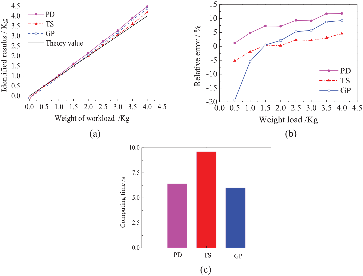
The workload predictions by dynamic model: (a) the absolute error of three methods for load identification, (b) the relative error of identified workload by three methods, and (c) the computational time of three methods for load identification.

As can be seen from Figure 6, the overall estimation of all data of a single group of experiments by the least square estimation method can improve the prediction accuracy of load. With the increase of experimental load, the absolute errors of the three load solving methods also increase. The torque method has good stability and accuracy, and the calculated load error is less than 0.1842 kg; Global parameter identification method only carries out dynamic calculation once, which depends more on the accuracy of experimental data, and the load error of robot obtained by it is less than 0.3706 kg. Among the three methods, the global identification method has the fastest speed and the torque solution method has the highest accuracy. The computer configuration of this example is AMD Ryzen 7 5800H. As can be seen from Figure 6(c), the load identification time of the three methods is long, which still cannot meet the requirements of real-time monitoring.

Load identification and analysis using improved Fourier neural network

Influence of frequency domain interception on recognition accuracy

In the proposed recognition method, K is the number of channels which is the key parameter to determine the truncation frequency of FNO_FFNN. It can retain the low frequency information to the network and extract important features. In order to analyze the process feature extraction by K value, this example sets K value to 4, 8, 12, 16, 20, and 24, and predicts the feature data with end load of 1–4 kg after 100 iterative training of the model. The prediction result and the average absolute error are shown in Figure 7.

Figure 7.

The influence of the setting of K value on the load identification error.

Taking four groups of loads as research examples, the variation law of load prediction accuracy with K value is shown in Figure 7. When the value of K is small, Fourier transform will cut off and discard the low frequency information, so that some useful feature information will be removed, resulting in a large load prediction error; With the gradual increase of K value, when the value is in an appropriate range, the error of load identification is low and stable, which shows that the characteristic information can be transmitted well between network layers. However, when the value of K is too large, the phenomenon of information over-fitting appears, which leads to the increase of load forecasting error.

Loss function curve analysis

The proposed method uses convolution to process the feature data and gradient descent principle to calculate the loss function. The smaller the loss value, the higher the training accuracy of the model. The evaluation function can characterize the accuracy of the output results of the model. The data used for model training are described as follows.

The maximum load of the UR5 robot is 5 kg. Here nine groups weight load with an equal interval are applied for pre-study, which are 0.5, 1, 1.5, 2, 2.5, 3, 3.5, 4, and 4.5 kg. Each group of the load is measured by 2400 points data with a sampling time interval 8 ms. For a point of the obtained data, it concludes nine dimensions value, such as actual position, actual velocity, actual current, target position, et al. To reduce the impact of random error, each group of the load testing is repeated 50 times for study.

The data of each load is divided into a training set and a test set with a ratio of 8 to 2. The loss function curve of FNO_FFNN training set and test set is shown in Figure 8. The loss function used in this paper is MSE (Mean Squared Error), and the evaluation function is LPLoss. The evaluation results of Fourier neural network model with 500 iterations are shown in the figure. The red and blue lines are the evaluation results of the model corresponding to the training data, and the downward trend of the loss function and the evaluation function is basically consistent, which shows that the learning accuracy of the model for the input data gradually increases in the iterative process. The black line is the evaluation result of the model corresponding to the test data. The loss function value fluctuates greatly in the first 250 iterations, and decreases slowly and tends to be stable after 250 iterations.

Figure 8.

The training set and test set loss function curve of FNO_FFNN.

The training process for the model is given in Figure 9.

Figure 9.

The training process for the model.

Influence of samples on load recognition effect

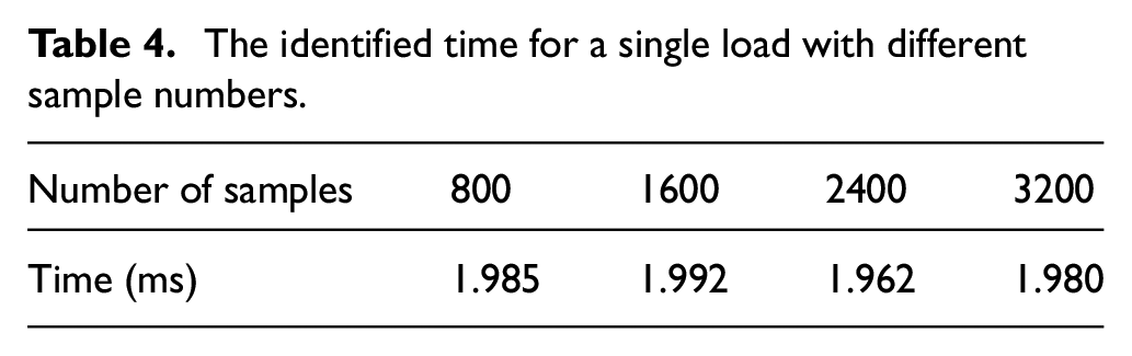
In order to analyze the influence of the number of samples on the accuracy and speed of load identification, the method of sub-sampling and data enhancement is adopted. The samples are set into four groups: 800, 1600, 2400, and 3200. The sub-sampling is to randomly reserve 2400 samples of the source data in the form of 1/2 and 1/4, and then bring the sampled data into the model for training. At the same time, every three rows and every six rows of the source data are averaged and added to the original sample data for data enhancement, and then the data are brought into the model for training. After the FNO_FFNN model is iteratively trained for 500 times, the characteristic data with an end load of 1–4 kg is predicted, and the prediction results and single load prediction time are shown in Table 4 and Figure 10.

Table 4.

The identified time for a single load with different sample numbers.

Number of samples	800	1600	2400	3200
Time (ms)	1.985	1.992	1.962	1.980

Figure 10.

The influence of the sample size on the load identification error: (a) the identified relative error with different sample sizes and (b) the average error and standard deviation with different sample sizes.

It can be seen from Figure 10(a) that the load prediction error will increase after sub-sampling, and large jump error may occur if important data points are missing. For example, when the sample size is 1600 in the figure, the error is larger than the sample size of 800, because the randomly removed samples contain more important data. When the enhancement sample is 3200, the average prediction error of the load is smaller than that of other groups, and its stability to all loads of the test group is also strong. It can be seen from Table 4 that the amount of sample data has little influence on the prediction time, and the prediction time of each group is within 2 ms, and the prediction speed of each sample group is 3000 times faster than that of the prediction method based on dynamics. Therefore, in this example, the enhanced data (the number of samples is 3200) is used as the characteristic data of subsequent model training. As shown in Figure 10(b), the average error and the standard deviation are greatest with a sample size 1600 because of the important data is missing. It is seem that the error average error and the standard deviation are became smaller with a bigger sample sizes.

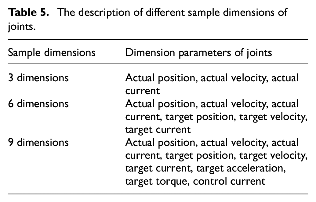
The sample data set used in this paper includes nine variables, including joint target position, velocity, acceleration, current, torque, actual position, actual velocity, actual current, and control current. The variable dimension number is set as three, six, and nine. Then the influence of sample dimensions on load prediction results is analyzed. The description of the sample dimensions of joints is given in Table 5 and the influence is shown in Figure 11.

Table 5.

The description of different sample dimensions of joints.

Sample dimensions	Dimension parameters of joints
3 dimensions	Actual position, actual velocity, actual current
6 dimensions	Actual position, actual velocity, actual current, target position, target velocity, target current
9 dimensions	Actual position, actual velocity, actual current, target position, target velocity, target current, target acceleration, target torque, control current

Figure 11.

The influence of the sample dimension on the load identification error and the training time: (a) identified error by different sample dimensions and (b) training time by different sample dimensions with samples size 2400.

It can be seen from the Figure 11 that when the sample dimension is reduced from 9 to 3, the relative prediction error increases more. As the weight load increases, the absolute value of the identified error decreases gradually. This is because random interference and other effects become smaller. In addition, if the sample dimension with other groups is applied, such as target position, target velocity, and target current, the identified load can not be predicted right.

Moreover, the error in a weight load 0.5 kg by sample dimension 6 is significantly greater than the results of the other two groups. Because the weight load of 0.5 kg is small and there is some random interference, the neural network falls into the local optimal solution when learning. This phenomenon disappears when the load increases. The average errors by the three groups are 13.83%, 5.06%, and 0.90%. It is seen in Figure 11(b) that as the data dimension increases, the training time does not increase much.

Load identification results and analysis

The maximum allowable load of UR5 robot is 5.0 kg. In order to ensure the safety, nine groups of standard load joint data of 0, 0.5, 1, 1.5, 2, 2.5, 3, 3.5, and 4t kg were collected experimentally. The improved Fourier network was used to train the sample data, and 81 groups of non-learning load data were set at an interval of 0.05 kg between 0 and 4 kg for testing and analysis.

Learning the standard load identification results in advance

The load characteristic data of standard parts are brought into the improved Fourier neural network model for 500 iterative training, and the load prediction results are shown in Figure 12.

Figure 12.

The standard load identified results by method of FNO_FFNN: (a) the identified results with standard weight load and (b) the relative error with standard weight load.

It can be seen from Figure 12 that the difference between the predicted load and the actual value of the improved Fourier neural network model is small, and its relative error is large when the load is small, which is caused by the discontinuity of the learning variables and the interference of uncertainty, but its absolute error is in an acceptable range. Secondly, compared with the prediction method based on dynamics, the prediction accuracy is greatly improved, which shows that Fourier neural network can effectively simulate the solution process of differential equations, especially for systems with strong nonlinearity, fuzzy model parameters or changing with running time, and its accuracy has certain advantages compared with the existing dynamic methods.

Non-pre-learning load identification results

The parameters of the network structure of the proposed model can be determined by sample learning of standard parts, so the accuracy is better when checking the learned load. In order to further study the generalization ability of the proposed method to any non-pre-learned load, 81 sets of loads between 0 and 4 kg are identified, and the results are shown in Figure 13.

Figure 13.

The load identification result by non-pre-learned: (a) the identified results and (b) the relative error result.

In Figure 13, the solid line is the theoretical value of load, and the dotted line is the predicted value of FNO_FFNN model. It can be seen that the proposed method has good prediction accuracy and stability for unknown load.

Comparison of prediction results using different models

In order to compare the prediction results of various neural networks, the method proposed in this paper is compared with representative neural network models such as FCN model, FFNN model, FNO model, and PINNs model, and the previous three dynamic models. Taking 2 kg as an example of pre-learning load, the analysis results of each model are shown in Table 6.

Table 6.

The analysis results by different models under 2 kg load.

Method	Identified result (kg)	Relative error (%)	Calculation time (ms)
TD	2.145	7.23	6400
TS	2.005	0.26	9600
GP	2.042	2.11	6000
FCN	2.063	3.12	0.602
FFNN	2.036	1.82	0.399
FNO	1.976	−1.18	1.895
FNO_FFNN	1.997	−0.10	1.980
PINNs	1.981	−0.93	0.722

It can be seen from the above table that it is a feasible method to solve the robot end load by using neural network. In terms of accuracy, the error of neural network method is smaller than that of dynamic method. In terms of speed, the time taken by neural network method to identify a load is only a few thousandths of that of dynamics, which has great advantages. For non-pre-learned loads, the prediction results are compared as shown in Figure 14. It can be seen from the figure that the FNO_FFNN method proposed in this paper has higher accuracy than the other four existing neural networks, which shows that its generalization ability is better.

Figure 14.

Comparison of analysis results by different models: (a) results of load identification by different models and (b) relative error of load identification by different models.

Method with variable channel number

In section “Influence of frequency domain interception on recognition accuracy,” the influence of the number of channels K on the identified accuracy of work load is given. It is seen that if the load is in different sections, such as small load range from 0 to 1.5 kg, medium load range from 1.5 to 3.5 kg, and heavy load 3.5 to 5 kg, the best choice of K value is not the same.²⁹ Here, an improved method with a variable K value is given as follows (Figure 15).

Figure 15.

Flow chart for the improved method by a variable K value.

The load identification results by the FNO_FFNN method the improved method are shown in Figure 16. It is seen from Figure 16(a) that the average value of all errors decrease from an initial value 0.038 kg by FNO_FFNN to 0.023 kg by improved method. Overall, the new method has smaller errors. As shown in Figure 16(b), owing to the random disturbance error, the ratio of relative error is relatively large if the weight load is small. When the weight load exceeds 0.5 kg, the relative error of identification is less than 3% by the improved method. In the range of the heavy load, the relative error is less than 2%.

Figure 16.

The load identification results by different methods with non-pre-learned: (a) the identified error of the weight load and (b) the relative error result.

Conclusion

In this paper, an improved Fourier neural network model is proposed to identify the real-time load of articulated robot. This method can effectively identify the parameters of high-dimensional system under the condition of local sample learning. The research results show that: (1) The efficiency of the improved Fourier neural network to identify a single load is more than 3000 times higher than that of solving the dynamic model, and the time to identify a single load can reach less than 2 ms. (2) When the number of samples is small or sub-sampling is applied for compressing the sample, a large jump error may occur if the important data features are missing. (3) Using the method proposed in this paper, the overall load identification error is less than 5% and the average load identification error is less than 2% under the non-pre-learning prediction samples. The larger the load, the higher the identification accuracy. (4) The use of improved methods can reduce relative errors by about 40%, and the random error value of the system under small load is also reduced.

The reduction of load identification errors has great significance in industrial applications. Firstly, it can improve the stability of robot operation by the accuracy identified load. The controller can calculate a more appropriate working torque for the joint. Secondly, the safety hazards decrease in dynamic operations. Accurate load recognition ensures that the robot moves more reliably when carrying heavy loads. Finally, the robot can identify the weight of goods during handling, match and screen special objects, and reduce the detection costs.

Footnotes

Handling Editor: Sharmili Pandian

Declaration of conflicting interests

The author(s) declared no potential conflicts of interest with respect to the research, authorship, and/or publication of this article.

Funding

The author(s) disclosed receipt of the following financial support for the research, authorship, and/or publication of this article: The paper is supported by the National Natural Science Foundation of China (No. 52205090 and No. 52275097), Guangdong HUST Industrial Technology Research Institute, Guangdong Provincial Key Laboratory of Manufacturing Equipment Digitization (2023B1212060012).

ORCID iD

Shangbin Long

References

Luo

An overview of calibration technology of industrial robots. IEEE CAA J Autom Sin 2021; 8(1): 23–36.

Liu

Tan

Long

SB.

Multi-axis fatigue load spectrum editing for automotive components using generalized S-transform. Int J Fatigue 2024; 188: 108503.

Liu

, et al. Fatigue reliability analysis and assessment of offshore wind turbine blade adhesive bonding under the coupling effects of multiple environmental stresses. Reliab Eng Syst Saf 2023; 238: 109426.

Spensieri

Åblad

Bohlin

, et al. Modeling and optimization of implementation aspects in industrial robot coordination. Robot Comput Integr Manuf 2021; 69: 102097.

Gao

Liu

, et al. Unsupervised meta learning with multiview constraints for hyperspectral image small sample set classification. IEEE Trans Image Process 2022; 31: 3449–3462.

Raissi

Perdikaris

Karniadakis

GE.

Physics-informed neural networks: a deeplearning framework for solving forward and inverse problems involving nonlinear partial differential equations. J Comput Phys 2019; 378: 686–707.

Zhang

, et al. Research on the operation and quality control of small rock hole shotcrete robot. Adv Mech Eng 2024; 16(6): 16878132241254960.

Falezza

Vesentini

Di Flumeri

, et al. A novel inverse dynamic model for 3-DoF delta robots. Mechatronics 2022; 83: 102752.

Wang

Sui

, et al. Alcoholism detection by data augmentation and convolutional neural network with stochastic pooling. J Med Syst 2018; 42(1): 1–11.

10.

Zhang

Satapathy

Zhu

, et al. A seven-layer convolutional neural network for chest CT based COVID-19 diagnosis using stochastic pooling. IEEE Sens J 2022; 22(18): 17573–17582.

11.

Nguyen

Ngo

BV.

A VGG-19 model with transfer learning and image segmentation for classification of tomato leaf disease. Agriengineering 2022; 4(4): 871–887.

12.

Wang

Zhang

, et al. Fixed-time adaptive fuzzy event-triggered control for uncertain nonlinear systems with output constraint and actuator failures. Fuzzy Sets Syst 2023; 467(15): 108563.

13.

Farsoni

Ferraguti

Bonfè

Safety-oriented robot payload identification using collision-free path planning and decoupling motions. Robot Comput Integr Manuf 2019; 59: 189–200.

14.

Pan

Jing

Jiao

, et al. A diagnosis framework for high-reliability equipment with small sample based on transfer learning. Complexity 2022; 2022: 1–15.

15.

Doan

Mai

, et al. A cluster-based data splitting method for small sample and class imbalance problems in impact damage classification. Appl Soft Comput 2022; 120: 108628.

16.

Raissi

Yazdani

Karniadakis

GE.

Hidden fluid mechanics: learning velocity and pressure fields from flow visualizations. Science 2020; 367(6481): 1026–1030.

17.

Zhu

Zabaras

Koutsourelakis

, et al. Physics-constrained deep learning for high-dimensional surrogate modeling and intangible quantification without labeled data. J Comput Phys 2019; 394: 56–81.

18.

Bar-Sinai

Hoyer

Hickey

, et al. Learning data-driven discretizations for partial differential equations. Proc Natl Acad Sci USA 2019; 116(31): 15344–15349.

19.

Kovachki

Azizzadenesheli

, et al. Fourier Neural Operator for Parametric Partial Differential Equations. International Conference on Learning Representations (ICLR), Virtual Conference, OpenReview net, 2021, pp. 1–16.

20.

Lample

Charton

. Deep learning for symbolic mathematics. In: International conference on learning representations (ICLR), Virtual Conference, OpenReview net, 2020, pp.1–24.

21.

Peng

Zhao

, et al. Multi-branch mutual-distillation transformer for EEG-based seizure subtype classification. IEEE Trans Neural Syst Rehabil Eng 2024; 32: 831–839.

22.

Yang

Chen

Xiao

, et al. Gaze and environmental context-guided deep neural network and sequential decision fusion for grasp intention recognition. IEEE Trans Neural Syst Rehabil Eng 2023; 31: 3687–3698.

23.

Chen

Cao

Chen

, et al. A fused deep fuzzy neural network controller and its application to pneumatic flexible joint. IEEE ASME Trans Mechatron 2023; 28(6): 3214–3225.

24.

Zang

Bao

, et al. Weak advisory networks for high-dimensional partial differential equations. J Comput Phys 2020; 411: 109409.

25.

Mathieu

Henaff

Lecun

. Fast Training of Constructive Networks through FFTs [C]//International Conference on Learning Representations (ICLR), Scottsdale, AZ, USA, 2013, pp. 1–9. IEEE

26.

Vahid

Prabhu

Farhadi

, et al. Butterfly transform: an efficient FFT based neural architecture design. In: 2020 IEEE/CVF conference on computer vision and pattern recognition (CVPR), Seattle, WA, USA, 13–19 June 2020, pp. 12021–12030. New York: IEEE.

27.

Raviola

Guida

De Martin

, et al. Effects of temperature and mounting configuration on the dynamic parameters identification of industrial robots. Robotics 2021; 10(3): 83.

28.

Universal Robots. DH parameters for calculations of kinematics and dynamics. 2022. https://www.universal-robots.com/articles/ur/application-installation/dh-parameters-for-calculations-of-kinematics-and-dynamics/

29.

Zhao

Wang

, et al. Data-driven learning for H∞ control of adaptive cruise control systems. IEEE Trans Veh Technol 2024; 73(12): 18348–18362.

A fast identification method for multi-joint robot load based on improved Fourier neural network

Abstract

Keywords

Introduction

Motivations

Literature reviews and objectives

Improved Fourier neural network

Fourier neural network

Network architecture

Operation principle

Improved Fourier neural network model

Improve the network architecture

Loss function

Model parameters

Test platform and data acquisition

Load identification experiment

Data acquisition and processing

Load identification and analysis based on dynamic model

Load dynamics modeling of robot

Torque linearization

Load dynamics identification results

Load identification and analysis using improved Fourier neural network

Influence of frequency domain interception on recognition accuracy

Loss function curve analysis

Influence of samples on load recognition effect

Load identification results and analysis

Learning the standard load identification results in advance

Non-pre-learning load identification results

Comparison of prediction results using different models

Method with variable channel number

Conclusion

Footnotes

Declaration of conflicting interests

Funding

ORCID iD

References