Sage Journals: Discover world-class research

Abstract

In order to coordinate a supply chain, reordering strategy of products must be synchronized. Meanwhile, the sequence of production and replenishment cycle time must be cost-effective. This article studies the economic lot and delivery scheduling problem with returns for a multi-stage supply chain in which each product is returned to manufacturing center by a constant rate of demand. Besides, there is a sub-open-shop system to remanufacture the returned items. The common cycle time and multiplier policies were adopted to accomplish the desired synchronization. For this purpose, a new mathematical model has been presented in which a manufacturer with the open-shop system purchases raw materials from suppliers and sends them to packaging companies after converting them into the final product. Since this is a nondeterministic polynomial time–hard problem, simulated annealing algorithms by heuristic methods and a biography-based optimization algorithm have been developed. For simulated annealing algorithm, two different scenarios have been proposed to solve the studied problem. Subsequently, numerical results with different scales have been applied to the problem. The numerical results show that biography-based optimization algorithm has a superb performance in finding the best solution for this problem.

Keywords

Economic lot size production scheduling open-shop system common cycle simulated annealing algorithm biography-based optimization algorithm

Introduction

In today’s competitive world, scheduling and inventory planning is a necessity for survival. Production planning and scheduling belong to two different stages of decisions: production planning in the medium term and scheduling in the short term. However, with the rise of competition in manufacturing stage and supply chains, coordination between the members of the chain depends on two major factors: scheduling and planning production and delivery. For this reason, research direction has been directed to determine the sequence of production and production planning and delivery simultaneously.

Combination of supply chain inventory control decisions with production sequence decisions is the most common known problem in the literature of the economic lot and delivery scheduling problem (ELDSP).¹ In this problem, it is important to establish a strategy that can coordinate inbound production scheduling and outbound deliveries throughout the supply chain. The overall objective is to reduce the inventory, production, and transportation costs throughout the supply chain. This problem is critical because it not only integrates different stages of the supply chain but also coordinates production and inventory decisions. The optimal solution has been obtained from a single supplier and a single assembler.^2–4

Creating common cycle increases the coordination between the existing echelons and enhances the ability of the supply chain to respond to unforeseen demands, as well as the efficiency of production designs compared to componential synchronization approach and semi-independent policies.⁵ Synchronization of the supply chains either through full or componential synchronization approach leads to some advantages for some members of the chain and some disadvantages for the others. The reason is that the different members at different stages have conflicting objectives. For example, suppliers with lower holding costs and higher setup costs seek to employ longer cycle time policies, while the common cycle policy is more desirable to those members of the supply chain with higher holding costs and lower setup costs. The studied supply chain includes three echelons. They include multiple suppliers and a production system, assembly, and packaging facilities located at the third stage.

It is assumed that each item is returned at a constant rate of demand to the manufacturing stage. This concept is inspired by Bae et al.⁶ Figure 1 represents the relationships between the production system elements for manufacturing and remanufacturing products.

Figure 1.

Manufacturing and remanufacturing system.⁶

Bae et al.⁶ believe that since manufacturing and remanufacturing operations are performed at the same production facility, two kinds of inventory are utilized to meet the demand: the serviceable inventory and the recoverable inventory. In order to omit this inventory, we propose an open-shop system with two kinds of separate machines, manufacturing and remanufacturing machines.

As an innovation, the open-shop system is considered for the second stage of supply chain and the use of a common cycle. In the open-shop system, each component should be placed on a certain number of machines, and there is no priority for the sequence of machines that should process the desired component. By these conditions, a group of machines is used for remanufacturing products.

In section “Literature review,” a summary of the literature on ELDSP is provided. Section “Problem description” describes a mathematical model. Simulated annealing (SA) algorithm is presented in section “SA algorithm,” and section “Biography-based optimization algorithm” discusses the results on the sample problems.

Literature review

The economic lot and production scheduling problem were first proposed in 1958 by Rogers. Basic assumptions of the problem included the presence of the one-stage process, the static demand and also the limited production capacity.⁵ Because of the complexity of the problem, in 1983, Hsu proved the complexity of the problem in nondeterministic polynomial time–hard (NP-hard) class.⁷

For the first time, Hahm and Yano examined the problem in a two-stage supply chain and considered the relationship between a customer and a supplier. They provided two heuristic algorithms under the common cycle policy. In the first algorithm, production and delivery cycle was assumed equal, but in the next algorithm, several deliveries were allowed during the production cycle.⁸

In 2000, Khouja expanded the work of Hahm and Yano.⁸ They added quality issues and rework cost of defective goods.⁹ In 2003, Khouja¹⁰ proposed some incentive mechanisms to encourage supply chain members to adopt the synchronization policy and the use of a common cycle.⁵ In 2003, Jensen and Khouja² presented an algorithm to solve ELDSP in polynomial time for a supplier and an assembler system considering inventory costs.

In 2005, Lee developed a new model at an infinite planning horizon in which he considered a producer with single-stage and single-product production system which purchased raw materials from suppliers and delivered them to customers after conversion to the final products. In fact, this model had a larger supply chain in which the supply of raw materials was also considered. The ultimate goal of the model was to obtain the optimal lot in the system without scheduling it.¹¹

Clausen and Ju developed the proposed algorithms of Hahm and Yano⁸ and presented a new hybrid algorithm in 2006 along with the heuristic algorithm. The proposed method has a less time for large-scale problems.¹²

Torabi et al. proposed a complex nonlinear binary model for ELDSP in a supply chain. The supply chain is made up of a common cycle product plant and assembly plant. The producer produces several items in a flexible linear production system and then assembly plant should assemble the items and deliver the products to the customers.³

In 2006, Kim et al. considered a three-stage supply chain in which a producer with single-stage system purchased raw materials and delivered them to its customers after converting those into final products. In their model, the producer works with single-stage multi-product production system under the common cycle approach. It should be noted that all products contain similar raw materials. At the end, an efficient heuristic algorithm was used to solve the model.⁴

The model that is allowed to run for mass flow in the supply area has been suggested by Torabi and Jenabi, in 2009. Mass flow has been used to minimize production time in a two-function supply chain.¹³

Osman and Demirli in two studies in 2010 and 2012 presented a quadratic model for ELDSP problem in a three-stage supply chain with a single-machine system. The model’s objective was to reduce all supply chain costs, and they introduced the common cycle as an essential factor of coordination in the chain.^1,14

In this regard, in 2013, Dousthaghi et al. presented a new model by encompassing a job shop production system. They considered irrelevant parallel machines and limited time horizon in their study. They developed a componential swarm optimization algorithm for the model and provided assumptions.¹⁵

In 2014, Kuhn and Liske provided a mathematical model and a detailed solution to ELDSP problem via two policies in maintaining and ordering goods at the manufacturing stage. Their exact solutions were studied and compared by two policies with the common cycle policy.¹⁶

Bae et al. presented a new formulation for time-varying lot sizing and scheduling by considering a single machine and returns. In this study, two kinds of inventory are assumed: serviceable inventory that holds manufactured products and revocable inventory that holds returned products, which needs remanufacturing. They presented a common cycle policy for this problem by mathematical modeling.⁶

In the literature, a few researches related to ELDSP in multi-stage supply chain with the aim of producing multiple products are presented. Also, not enough attention has been paid to the open-shop system in the literature. For this reason, in this article, a new mathematical model is proposed for the problem with regard to the open-shop system in a supply chain. In order to solve the model, an SA algorithm is also used to achieve satisfactory solutions in less time. The distinction to other previous studies is to present a new mathematical model to optimize production and delivery in three echelon supply chain. Since this is a new mathematical model, the customized optimization methods used in this study were not seen in other researches.

Problem description

For the manufacturers, optimizing the inventory system alone cannot reduce their wide range of costs. Accordingly, attention to the policy of purchasing raw materials, holding items, and delivering products together is necessary, and in this situation, surveying the whole supply chain products and the scheduling of items delivery is a must.

In this article, production system with the common cycle is proposed. To meet the customers’ demand, this must be deployed within the supply chain. The concept through which the system is deployed is the full synchronization of the supply chain.

Common cycle time synchronization approach is recommended to respond quickly to the changes in the demand-production market. In this case, the system simultaneously makes decisions on reordering cycle time at each stage of the supply chain in line with the production sequence. Such an approach in relation to planning can be cost-effective for the supply chain.

In addition to determining common cycle time, production sequence in every supplier and in the manufacturing system is the decision variable. In order to model ELDSP problem in a three-stage supply chain, the following assumptions have been made:

All stages work at the same cycle time (T), which is the model’s decision variable.

Each supplier in the first stage of supply chain has a single production line.

At the manufacturing center (T₁), products in the open-shop production system are processed by two kinds of machines (manufacturing and remanufacturing).

All products at the end of the period (T) are distributed to the next stage by one shipment.

The sent shipment is equal to the demand of the next stage.

With the move from primary stages to the end of the chain, holding costs of items get increased because of the added value of the components of the product.

The ordering policy is adapted to economic order quantity (EOQ) in all stages of the supply chain.

In the open-shop system, to prepare the machine to process the next item, this item does not need to be produced by the previous machine.

The assembly company reveals defect items and returns them to the manufacturing center. Relying on historical data, the rate of returned items is constant.

In the manufacturing center, we have a sub-open-shop system for manufacturing items and another sub-open shop for remanufacturing returned items. Figure 2 shows the structure of the three stages of the supply chain.

Figure 2.

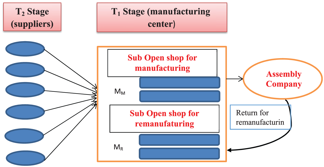
Three-stage structure of the supply chain under study.

Indexes

k: index of supplier T₂

i, b: index of items at each stage of the chain

q: index of production sequence at T₂ stage

h, m: index of machines in the open-shop system

$M_{m} \subset M$ : machines in manufacturing center for manufacturing

$M_{R} \subset M$ : machines in manufacturing center for remanufacturing

Parameters

n_k: number of the kth items of T₂

J: total number of items of the T₁

$h_{ki}^{r}$ : holding cost of each unit of ith item as the raw material in kth supplier (T₂) per time unit

$h_{ki}^{f}$ : holding cost of each unit of ith item as the final product in kth supplier (T₂) per time unit

$h_{i}^{r}$ : holding cost of each unit of ith item as the raw material (final produced in T₂) in manufacturing center per time unit

$h_{i}^{f}$ : holding cost of each unit of ith item as the final product in manufacturing center per time unit.

$h_{ai}$ : holding cost of each unit of ith item at the assembly company per time unit

$D_{ki}$ : demand of ith item in kth supplier (T₂)

$D_{i}$ : demand of ith item in manufacturing center (T₁)

$D_{a}$ : demand of assembled product

$P_{ki}$ : production rate of ith item in kth supplier

$P_{im}$ : production rate of ith item in machine m of the manufacturing center

$S_{ki}$ : setup time of production of ith item in kth supplier

$S_{im}$ : setup time of production of ith item in machine m of the manufacturing center

$B_{ki}$ : cost of preparation of ith item in kth supplier

$B_{im}$ : cost of setup for ith item in machine m of manufacturing center

$A_{k}$ : shipment cost of each unit delivered at in kth supplier

$A_{c}$ : shipment cost of each unit delivered at manufacturing center

$A_{a}$ : shipment cost of each unit delivered at the assembly company

$β_{i}$ : constant return rate of ith item

Decision variables

T: common cycle time of the entire chain

$X_{kiq}$ : binary variable that is equal to 1 when ith item is placed in sequence q in kth supplier

$X_{ibm}$ : binary variable that is equal to 1 when ith item is processed on machine m before bth item

$y_{imh}$ : binary variable that is equal to 1 when ith item processing on machine m is earlier than hth item in the manufacturing center

$TS M_{im}$ : start time of processing ith item on machine m in the manufacturing center

$TS R_{im}$ : start time of processing ith item on machine m for remanufacturing in the manufacturing center

$TF M_{i}$ : finishing time of processing ith item in the manufacturing center

$TF R_{i}$ : finishing time of remanufacturing ith item in the manufacturing center

Mathematical model

M i n T c = \sum_{k = 1}^{K} [\sum_{i = 1}^{n_{k}} h_{k i}^{r} \sum_{q = 1}^{n_{k}} (\frac{T D_{k i}^{2}}{2 P_{k i}} X_{k i q} + D_{k i} X_{k i q} \times (S_{k i} + \sum_{\begin{matrix} b = 1 \\ b \neq i \end{matrix}}^{n_{k}} \sum_{l = 1}^{q - 1} X_{k b l} (S_{k b} + \frac{T D_{k b}}{P_{k b}})))

(1-1)

+ \sum_{i = 1}^{n_{k}} h_{ki}^{f} \sum_{q = 1}^{n_{k}} (\frac{{TD}_{ki}^{2}}{2 P_{ki}} X_{kiq} + D_{ki} X_{kiq} \sum_{\binom{b = 1}{b \neq i}}^{n_{k}} \sum_{l = q + 1}^{n_{k}} X_{kbl} (S_{kb} + \frac{T D_{kb}}{P_{kb}}))]

(1-2)

+ \sum_{m_{1}, m_{2} \in M_{R}} \sum_{i = 1}^{J} h_{i}^{r} (TS M_{i m_{1}} y_{i m_{1} m_{2}} + TS M_{i m_{2}} y_{i m_{2} m_{1}}) + h_{i}^{f} (T - TF M_{i})

(1-3)

+ \sum_{m_{1}, m_{2} \in M_{M}} \sum_{i = 1}^{J} β_{i} [h_{i}^{f} (TS R_{i m_{1}} y_{i m_{1} m_{2}} + TS R_{i m_{2}} y_{i m_{2} m_{1}}) + h_{i}^{f} (T - TF M_{i})]

(1-4)

+ \sum_{i = 1}^{n_{a}} D_{ai} h_{ai} \frac{T}{2} + \frac{1}{T} (\sum_{k = 1}^{K} (A_{k} + \sum_{i = 1}^{n_{k}} B_{ki}) + (\sum_{i = 1}^{J} \sum_{m = 1}^{2} B_{im}) + A_{c} + A_{a})

(1-5)

Subject to

\sum_{i = 1}^{n_{k}} (S_{ki} + \frac{D_{ki}}{P_{ki}} T) \leq T, k = 1, 2, \dots, K

(2)

\sum_{q = 1}^{n_{k}} X_{kiq} = 1, k = 1, 2, \dots, K; i = 1, 2, \dots, n_{k}

(3)

\sum_{i = 1}^{n_{k}} X_{kiq} = 1, k = 1, 2, \dots, K; q = 1, 2, \dots, n

(4)

\begin{array}{l} T S M_{i m_{1}} \leq T S M_{i m_{2}} + M (1 - y_{i m_{1} m_{2}}), \\ i = 1, 2, …, J; m_{1}, m_{2} \in M_{m} \end{array}

(5)

\begin{array}{l} T S M_{i m_{2}} \leq T S M_{i m_{1}} + M (1 - y_{i m_{2} m_{1}}), \\ i = 1, 2, …, J; m_{1}, m_{2} \in M_{m} \end{array}

(6)

\begin{array}{l} T S R_{i m_{1}} \leq T S R_{i m_{2}} + M (1 - y_{i m_{1} m_{2}}), \\ i = 1, 2, …, J; m_{1}, m_{2} \in M_{R} \end{array}

(7)

\begin{array}{l} T S R_{i m_{2}} \leq T S R_{i m_{1}} + M (1 - y_{i m_{2} m_{1}}), \\ i = 1, 2, …, J; m_{1}, m_{2} \in M_{R} \end{array}

(8)

\begin{array}{l} T S M_{i m_{1}} + S_{i m_{1}} + \frac{D_{i}}{P_{i m_{1}}} T - M (1 - y_{i m_{1} m_{2}}) \leq T S M_{i m_{2}} + S_{i m 2}, \\ i = 1, 2, …, J; m_{1}, m_{2} \in M_{M} \end{array}

(9)

\begin{array}{l} T S M_{i m_{2}} + S_{i m_{2}} + \frac{D_{i}}{P_{i m_{2}}} T - M (1 - y_{i m_{2} m_{1}}) \leq T S M_{i m_{1}} + S_{i m 1}, \\ i = 1, 2, …, J; m_{1}, m_{2} \in M_{M} \end{array}

(10)

\begin{array}{l} T S R_{i m_{1}} + S R_{i m_{1}} + β_{i} \frac{D_{i}}{P_{i m_{1}}} T - M (1 - y_{i m_{1} m_{2}}) \leq T S R_{i m_{2}} + S_{i m 2}, \\ i = 1, 2, …, J; m_{1}, m_{2} \in M_{R} \end{array}

(11)

\begin{array}{l} T S R_{i m_{2}} + S_{i m_{2}} + β_{i} \frac{D_{i}}{P_{i m_{2}}} T - M (1 - y_{i m_{2} m_{1}}) \leq T S R_{i m_{1}} + S_{i m 1}, \\ i = 1, 2, …, J; m_{1}, m_{2} \in M_{R} \end{array}

(12)

TS M_{im} + S_{im} + \frac{D_{i}}{P_{i}} T \leq TF M_{i}, i = 1, 2, \dots, J; m \in M_{M}

(13)

TS R_{im} + S_{im} + β_{i} \frac{D_{i}}{P_{im}} T \leq TF R_{i}, i = 1, 2, \dots, J; m \in M_{R}

(14)

TF M_{i} \leq T, i = 1, 2, \dots, J

(15)

TF R_{i} \leq T, i = 1, 2, \dots, J

(16)

\begin{array}{l} y_{i m_{1} m_{2}} + y_{i m_{2} m_{1}} = 1, \\ i = 1, 2, …, J; m_{1}, m_{2} \in M_{m}; m_{1} \neq m_{2} \end{array}

(17)

\begin{array}{l} y_{i m_{1} m_{2}} + y_{i m_{2} m_{1}} = 1, i = 1, 2, …, J; \\ m_{1}, m_{2} \in M_{R}; m_{1} \neq m_{2} \end{array}

(18)

\begin{array}{l} X_{i b m} + X_{b i m} = 1, i = 1, 2, …, J; \\ b = 1, 2, …, J; b \neq i; m \in M_{M} \end{array}

(19)

\begin{array}{l} X_{i b m} + X_{b i m} = 1, i = 1, 2, …, J; \\ b = 1, 2, …, J; b \neq i; m \in M_{R} \end{array}

(20)

\begin{array}{l} X_{k i q} \in {0, 1}, k = 1, 2, …, K; \\ i = 1, 2, …, n_{k}; q = 1, 2, …, n_{k} \end{array}

(21)

\begin{array}{l} X_{i b m} \in {0, 1}, i = 1, 2, …, J; \\ b = 1, 2, …, J; m = 1, 2 \end{array}

(22)

y_{imh} \in {0, 1}, i = 1, 2, \dots, J; m = 1, 2; h = 1, 2

(23)

T S_{im} \geq 0, i = 1, 2, \dots, J; m = 1, 2

(24)

TF M_{i} \geq 0, i = 1, 2, \dots, J

(25)

TF R_{i} \geq 0, i = 1, 2, \dots, J

(26)

T \geq 0

(27)

The objective function represents the total cost of the supply chain. The first term of objective function represents holding cost for unprocessed items and setup cost in suppliers. The second term denotes the holding cost for the processed items in suppliers. The third term represents holding cost for unprocessed and processed items in the manufacturing center. The fourth term shows the above concept for remanufacturing items, and the fifth term represents the cost of shipment of items between stages of the supply chain (for more detail, see Osman and Demirli¹).

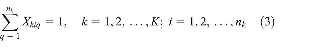
Constraint 2 states that at each supplier, the total time of item setup and manufacturing should not be more than the cycle time. Constraint 3 states that at each supplier, each item should be placed at one production sequence station. Constraint 4 states that at each supplier, one item must be placed in each production sequence station. Other constraints are related to the open-shop system at the manufacturing center.

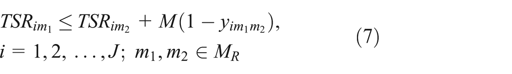
Constraints 5 and 6 show the sequence of production on manufacturing machines. Constraints 7 and 8 show the sequence of production on remanufacturing machines. Constraints 9 and 10 state that for each item, the finishing time of processing on the first machine is less than the start and setup time of the component on the second machine. It means that it is possible that setting up the second machine for an item can be done before finishing its processing on the first machine.

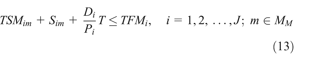
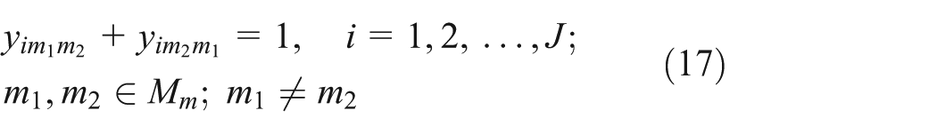
Constraints 11 and 12 have a similar concept to constraints 9 and 10 for remanufacturing items. Constraints 13 and 14 determine finishing time of item processing. Constraints 15 and 16 indicate that finishing time of processing for all items must be less than the cycle time. Constraints 17 and 18 show the sequence capability in the open-shop system for manufacturing and remanufacturing. Constraints 19 and 20 show the precedence between two activities on a machine in the open-shop system. Constraints 21–27 also specify the type of decision variables.

SA algorithm

The simulated algorithm is a simple and effective meta-heuristic algorithm for solving optimization problems.¹⁷ This approach moves toward the optimal solution by stepwise creation and evaluation of successive results. To move, a new neighborhood is randomly generated and evaluated. In this way, the points near the given point are evaluated in the search space. If the new point is a better point (reduces cost function), it is selected as the new point in the search space, and if gets worse (increases the cost function), it is also selected based on a probabilistic function. In simpler words, for the minimization of the cost function, the search is always done to lower the amount of cost function, but it is possible that the movement sometimes contributes to an increase in the cost function. The next point is usually adopted by a measure called Metropolis criteria

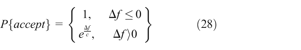
P {accept} = {\begin{matrix} 1, & Δ f \leq 0 \\ e^{\frac{Δ f}{c}}, & Δ f 〉 0 \end{matrix}}

(28)

where P is the probability of adopting the next point, $Δ f$ is the changes in objective function for the given neighborhood, and C is the control parameter considered to be equal to the current temperature. To stop the algorithm, a stopping criterion is required. A criterion for this purpose can be reaching the final temperature. Another criterion can be a lack of obtaining better results in a specific number of repetitions.

In this study, for the solved instances, the initial temperature is 1000, and the temperature reduction rate is 0.01 of the temperature at the previous stage. In other words, $T_{i + 1} = 0.99 T_{i}$ , and the stopping criterion is the lack of improvements in 100 recent repetitions or reaching a temperature of less than 1.

Local searches

In order to employ the SA for this problem and to create a neighborhood in SA algorithm, two types of changes in the solutions (local searches) are considered. These changes are called as first type local search and second type local search.

In the first type local search, production sequence is changed at the T₂ stage, and if appropriate to the change in the common cycle of the supply chain, the change is unacceptable (constraint 2 is violated), and it will increase up to an acceptable level. The second type local search is exactly the same process for the production sequence in the open-shop system at the manufacturing center.

Adoptive SA

Two scenarios are presented to evaluate the performance of SA algorithm. In the first scenario (SA I), SA algorithm runs only by regarding the generation of the first type local search. After this, the SA algorithm runs again with the difference that the output of the first implementation is considered as the initial solution and using the second type of local search. In Figure 3, the structure of SA I has been cleared.

Figure 3.

The structure of SA I.

In the second scenario (SA II), SA algorithm runs once. In this case, two local search methods are used at the same time, so that at iteration of SA algorithm, one of the two local search methods is selected and runs randomly with 50% chance. This kind of SA is shown in Figure 4.

Figure 4.

The structure of SA II.

Biography-based optimization algorithm

In 2008, D Simon¹⁸ used biography science, the science of studying geographical distribution of species and its mathematics to solve optimization problems, and proposed a new intelligent method called biography-based optimization (BBO). This method has common characteristics with other biology-based optimization methods such as genetic algorithm (GA) and particle swarm optimization. BBO is a population-based evolutionary algorithm that is inspired by animals and birds migration between islands. In fact, the biography science is the science of studying geographical distribution of species. Islands that are proper places for species to live have high habitat suitability index (HSI). Characteristics that determine HSI include factors such as rainfall, herbal diversity, topographic characteristics, area soil, and temperature, which are called suitability index variable (SIV).

The islands with high HSI have low immigration rate because they are already filled with other species and cannot accept new ones. As the islands with low HSI have low population, their immigration rate is high. Because suitability of a place is proportional to its biographical diversity, immigration of new species to place with high HSI may lead to an increase of that area’s HSI. Similar to other evolutionary algorithms like GA that has operators such as mutation operator and cut operator, in BBO, migration and mutation operators cause desired changes in the procedure of generations’ population.

Migration operator

Assume that we have a problem and a set of candidate solutions that are represented by an array of integers. We can consider each integer in the solution array as an SIV (similar to a gene in GA method). Moreover, assume that there are methods to determine desired solutions. Desired solutions have high HSI (habitats with high species), and weak solutions have low HSI (habitats with low species). The HSI in BBO is similar to fitness function in other population-based optimization algorithms.

Each habitat (solution) has immigration rate λ and emigration rate µ, which are used to share information between solutions stochastically. These rates are calculated using the following equations

λ_{i} = I (1 - \frac{k (i)}{n})

(29)

μ_{i} = E (\frac{k (i)}{n})

(30)

where I and E are the maximum immigration rate and emigration rate, respectively, and k(i) is the number of species in habitat i. k(i) is a number between 1 and n, where n is a number of population members (n for the best solution and 1 for the worst solution). Each solution is modified with respect to other solutions with a probability. If a solution is selected for modification, we use immigration rate (λ) to determine stochastically whether each of SIVs should be modified or not. If an SIV in solution Si is selected for modification, using emigration rate (µ) of other solutions, we decide stochastically which solution must cause to the migration of an SIV, which is selected stochastically, to solution Si.

Mutation operator

Sudden changes may lead to change in the HSI of a habitat. Moreover, such changes may cause differences in a number of species with the balanced value (unnatural substances that are brought from neighbor habitats by the water, diseases, natural disasters, etc.). We model this as mutation of SIV in the BBO. It should be noted that probability of a number of species in the habitat is used to determine mutation rate

m (s) = m_{max} (\frac{1 - P_{s}}{P_{max}})

(31)

where m_max is the maximum mutation rate and is defined by the user and P_s is the probability of having s species in the habitat.

Numerical results

In order to validate the proposed model and evaluate the performance of the proposed algorithms, the model was coded in GAMS software. The SA and BBO have also been coded in MATLAB 2014. Then, six random examples at small scale and six examples at medium and large scales were generated and implemented by GAMS software and the presented algorithms. Data of the generated problems are shown in Tables 1 and 2.

Table 1.

Generated problems at small scale.

Problem	Suppliers	Items
1	2	3
2	3	5
3	4	8
5	5	10
6	10	15

Table 2.

Generated problems in a large scale.

Problem	T₂ suppliers	Components
7	15	20
8	20	30
9	25	50
10	30	100
11	35	150
12	40	200

Holding costs at each stage are considered between 1 and 10 so that the holding cost of raw materials is less than that of the final product. Component production rates are considered between 5 and 10 randomly, and demand rate is determined by discrete uniform distribution between 4 and 8. Setup times are determined by uniform distribution between 0.5 and 1, and the cost of setting up by the same distribution of about 50–100. Finally, the shipment costs are also generated from a uniform distribution of about 20 and 50.

Each of the examples generated at the small scale has been implemented by GAMS software and time limit of 3600 s and also by software MATLAB 2014 using SA under two different scenarios and BBO algorithm. The result summary is presented in Table 3.

Table 3.

The result summary of the implementation of problems at small scale.

Problem	GAMS		SA I			SA II			BBO
Problem	Z	T	Z	(T₁ + T₂)/2	GAP (%)	Z	T	GAP (%)	Z	T	GAP (%)
1	59.3	3.7	59.3	1.2	0	59.3	1.4	0	59.3	1.9	0
2	69.1	29.4	69.1	4.5	0	69.1	3.7	0	69.1	4.2	0
3	127.6	108.7	137.9	12.4	7.47	134.4	10.1	5.06	127.6	11.3	0
4	159.3	867.2	166.3	11.9	4.21	165.7	14.5	3.86	161.1	14.1	1.12
5	249.6	1937.1	251.4	27.3	0.72	254.1	26.8	1.77	255.3	27.5	2.23
6	561.9	3600	590.1	39.1	4.78	581.3	34.6	3.34	572.9	35.1	1.92
Average	−	1091.02	−	16.066	2.863	−	15.1833	2.338	−	15.683	0.878

SA: simulated annealing; BBO: biography-based optimization.

In Table 3, Z is the obtained value of the objective function, and T shows the execution time in seconds. For the first scenario of SA, the average time of two runs has been reported. GAP shows the proposed algorithms difference rate by optimal solution and computed by equation (32)

GAP = \frac{Z_{algorithm} - Z_{optimum}}{Z_{algorithm}} \times 100

(32)

As can be seen, GAMS software can solve only five problems in less than 1 h. The average solving time for SA algorithm for the first scenario is about 16 s and about 15 s for the second scenario. Also, the average execution time for BBO is about 15 s. It means that the proposed algorithms have equal solving time approximately. In terms of the GAP, the second scenario has lower error rate than the first scenario of SA. In addition, the BBO algorithm has better performance on this criterion when compared with SA.

Since GAMS software cannot provide an optimal solution within the reasonable time for these problems, the comparison is only performed between the two scenarios of SA and that of BBO algorithm. Summary results for solving large-scale problems are given in Table 4.

Table 4.

Results of solving six large-scale problems.

Problem	SA I			SA II			BBO
Problem	Z	(T₁ + T₂)/2	GAP (%)	Z	T	GAP (%)	Z	T	GAP (%)
7	811.3	53.6	0	816.4	41.2	0.62	817.9	52.95	0.81
8	1276.1	59.4	2.01	1250.4	50.9	0	1254.1	53.77	0.3
9	2864.3	60.4	0.13	2869.3	62.7	0.31	2860.5	69.48	0
10	4853.7	97.5	0	4860.9	80.1	0.15	4871.3	104.13	0.36
11	5379.2	124.3	9.81	5300.7	131.9	8.47	4851.5	140.95	0
12	7394.8	186.4	0.2	7388.4	179.5	0.11	7380.3	185.73	0
Average	−	96.9333	2.025	−	91.05	1.61	−	101.168	0.245

SA: simulated annealing; BBO: biography-based optimization.

As shown in Table 4, the second scenario of SA could perform better in three out of six problems than the first scenario of it; however, the GAP rate of the first scenario of SA in obtained solutions (best solution) was higher than that of the second scenario so that the average GAP rate for the second scenario was 1.6% and for the first scenario 2.0%. In these situations, BBO algorithm has less than 1% GAP. It means that this algorithm has better operations to find the optimum solution. In the case of execution time, the first scenario of SA has a difference of about 4 s with the second scenario of it, and BBO algorithm has about 10 s more. It means that in order to find a better solution by BBO, it needs more time than SA algorithm. Execution time diagram for the two SA scenarios and BBO algorithm of the 12 solved problems is shown in Figures 5 and 6.

Figure 5.

Execution time for the two scenarios of SA and BBO.

Figure 6.

Bar chart for execution time.

As shown in Figure 6, both scenarios of SA have nearly similar action in terms of time, and BBO algorithm needs a few more time to present its best solution. However, the average time of solution for SA algorithm in the second scenario is less than that of the first scenario.

Conclusion

In this article, to solve the economic lot and delivery scheduling problem with returns (ELDSPR) problem, a new mathematical model was presented in a three-stage supply chain. In this model, the common cycle approach was used to coordinate the supply chain. Also, the given production system at the second stage of the chain considered the open-shop system. In this production system, a group of machines have to manufacture items, and others should remanufacture returned items. To solve the proposed model, an SA algorithm and a BBO algorithm were developed. In order to evaluate the performance of SA algorithm, two scenarios were presented regarding the structure of the algorithm and compared with BBO algorithm in terms of time and GAP rate. The results show that the BBO algorithm can be introduced as a convenient and efficient way of solving the ELDSPR optimization problem in a supply chain.

Footnotes

Academic Editor: Wu Naiqi

Declaration of conflicting interests

The author(s) declared no potential conflicts of interest with respect to the research, authorship, and/or publication of this article.

Funding

The author(s) received no financial support for the research, authorship, and/or publication of this article.

References

Osman

Demirli

Economic lot and delivery scheduling problem for multi-stage supply chains. Int J Prod Econ 2012; 136: 275–286.

Jensen

Khouja

An optimal polynomial time algorithm for the common cycle economic lot and delivery scheduling problem. Eur J Oper Res 2004; 156: 305–311.

Torabi

Ghomi

Karimi

A hybrid genetic algorithm for the finite horizon economic lot and delivery scheduling in supply chains. Eur J Oper Res 2006; 173: 173–189.

Kim

Hong

Chang

SY.

Joint economic procurement—production–delivery policy for multiple items in a single-manufacturer, multiple-retailer system. Int J Prod Econ 2006; 103: 199–208.

Sarker

Newton

A genetic algorithm for solving economic lot size scheduling problem. Comput Ind Eng 2002; 42: 189–198.

Bae

Moon

Yun

A time-varying lot sizes approach for the economic lot scheduling problem with returns. Int J Prod Res 2016; 54: 3380–3396.

Hsu

. On the general feasibility test of scheduling lot sizes for several products on one machine. Manage Sci 1983; 29(1): 93–105.

Hahm

Yano

CA.

The economic lot and delivery scheduling problem: models for nested schedules. IIE Trans 1995; 27: 126–139.

Khouja

The economic lot and delivery scheduling problem: common cycle, rework, and variable production rate. IIE Trans 2000; 32: 715–725.

10.

Khouja

Synchronization in supply chains: implications for design and management. J Oper Res Soc 2003; 54: 984–994.

11.

Lee

A joint economic lot size model for raw material ordering, manufacturing setup, and finished goods delivering. Omega 2005; 33: 163–174.

12.

Clausen

A hybrid algorithm for solving the economic lot and delivery scheduling problem in the common cycle case. Eur J Oper Res 2006; 175: 1141–1150.

13.

Torabi

Jenabi

Multiple cycle economic lot and delivery-scheduling problem in a two-echelon supply chain. Int J Adv Manuf Tech 2009; 43: 785–798.

14.

Osman

Demirli

A bilinear goal programming model and a modified Benders decomposition algorithm for supply chain reconfiguration and supplier selection. Int J Prod Econ 2010; 124: 97–105.

15.

Dousthaghi

Tavakkoli-Moghaddam

Makui

Solving the economic lot and delivery scheduling problem in a flexible job shop with unrelated parallel machines and a shelf life by a proposed hybrid PSO. Int J Adv Manuf Tech 2013; 68: 1401–1416.

16.

Kuhn

Liske

An exact algorithm for solving the economic lot and supply scheduling problem using a power-of-two policy. Comput Oper Res 2014; 51: 30–40.

17.

Kirkpatrick

Optimization by simulated annealing: quantitative studies. J Stat Phys 1984; 34: 975–986.

18.

Simon

Biogeography-based optimization. IEEE T Evolut Comput 2008; 12: 702–713.

A new production and delivery scheduling problem with common cycle in a supply chain with open-shop system and returns

Abstract

Keywords

Introduction

Literature review

Problem description

Indexes

Parameters

Decision variables

Mathematical model

SA algorithm

Local searches

Adoptive SA

Biography-based optimization algorithm

Migration operator

Mutation operator

Numerical results

Conclusion

Footnotes

Declaration of conflicting interests

Funding

References