A Simulated Annealing-Based Heuristic Algorithm for Job Shop Scheduling to Minimize Lateness

Abstract

A decomposition-based optimization algorithm is proposed for solving large job shop scheduling problems with the objective of minimizing the maximum lateness. First, we use the constraint propagation theory to derive the orientation of a portion of disjunctive arcs. Then we use a simulated annealing algorithm to find a decomposition policy which satisfies the maximum number of oriented disjunctive arcs. Subsequently, each subproblem (corresponding to a subset of operations as determined by the decomposition policy) is successively solved with a simulated annealing algorithm, which leads to a feasible solution to the original job shop scheduling problem. Computational experiments are carried out for adapted benchmark problems, and the results show the proposed algorithm is effective and efficient in terms of solution quality and time performance.

1. Introduction

Scheduling has been an important research field in robotics and computer-integrated manufacturing [22, 8]. The job shop scheduling problem (JSSP) is one of the most frequently adopted models in the area of scheduling research [15, 2, 16, 11]. However, most variants of JSSP are $\mathcal{N}\mathcal{P}$ -hard in the strong sense and thus defy ordinary solution methods. Enumerative approaches, such as the branch-and-bound algorithm [7], can only conquer small-scale problem instances. The most common heuristic methods devised in the early days include dispatching rules [17, 10, 3] and shifting bottleneck [1, 4, 12]. In recent years, meta-heuristic algorithms, such as simulated annealing (SA) [26], genetic algorithms (GA) [28], scatter search (SS) [18], tabu search (TS) [27] and particle swarm optimization (PSO) [25], have clearly become the research focus in practical optimization methods for solving ordinary-scale JSSPs.

However, the size of JSSPs in practical manufacturing environments is much larger than in theoretical research. In this case, the solution space is too large to be searched effectively by simple meta-heuristics. To address this difficulty, several decomposition-based algorithms have been proposed [19, 5, 21, 20, 23], which decompose the original large-scale problem into a series of smaller problems (subproblems) and finally obtain a solution to the original problem after these subproblems are solved respectively. But there are some drawbacks with these existing approaches. The decomposition algorithm proposed in [19, 20] has exponential complexity and thus cannot be directly applied to large-scale problems; the algorithm in [5] encounters deterioration in solution quality because it adds extra constraints to each subproblem; the method presented in [21] does not guarantee the feasibility of subproblem solutions for the original problem and relies on a heuristic coordination algorithm to construct a feasible solution for the original problem.

In this paper, we propose a decomposition-optimization algorithm based on simulated annealing (DOASA) to solve large-scale JSSPs with the objective of minimizing maximum lateness. In DOASA, the original problem will be divided into several subproblems, each of which corresponds to a subset of operations. The subproblems are first determined and then successively solved by two optimization processes, both of which are implemented with simulated annealing in order to save computational time. Before decomposition, the constraint propagation technique is applied as a preprocessor on the original problem so that some disjunctive arcs can be resolved. This information provides guidance for the determination of decomposition policy and subproblems.

The paper is organized as follows. The discussed job shop scheduling problem is formulated in Section 2. Section 3 introduces the important tools that are used by our algorithm. Section 4 describes the DOASA in detail. The computational results are provided in Section 5. Finally, some conclusions are given in Section 6.

2. Problem formulation

In a JSSP instance, a set of n jobs ${\{J_j\}}_{j=1}^n$ are to be processed on a set of m machines ${\{M_k\}}_{k=1}^m$ such that each machine can process only one job at a time, and each job may be processed by only one machine at a time. Each job has a fixed processing route which traverses all the machines in a predetermined order. A preset due date is given for each job. Since due date related criteria are of much greater concern in practical scheduling, maximum lateness is adopted as the optimization objective.

JSSP can be described by a disjunctive graph $G(N\mathrm{,}C\mathrm{,}D)$ [23]. $N=O\cup \{\mathrm{0,}\ast \}$ is the set of nodes where $O=\{\mathrm{1,2,}\dots \mathrm{,}n\times m\}$ are associated with the $n\times m$ operations of the JSSP instance. 0 and ∗ denote the dummy source node and the dummy sink node, respectively. C is the set of conjunctive arcs which connect successive operations of the same job. Thus, C models the technological constraints in the JSSP instance. $D={\displaystyle {\cup }_{k=1}^m}{D}_k$ is the set of disjunctive arcs if $D_k$ is used to denote the disjunctive arcs that correspond to the operations on machine k. $D_k$ contains the arcs that connect each pair of operations to be processed by machine k and require that these operations cannot be processed simultaneously. Therefore, the directions of the disjunctive arcs are yet to be determined. Finding a feasible schedule for JSSP is equivalent to orienting all the disjunctive arcs without causing any directed cycles in the resulting graph. The weight of each arc equals the processing time of the operation that is associated with the tail of the arc.

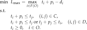
The discussed JSSP can be formulated as follows:

$\begin{array}{ll}\min \hspace{0.17em}\hspace{0.17em}\hfill & L_{\max }=\underset{i\in F(O)}{{\displaystyle \max }}\left\{t_i+p_i-d_i\right\}\hfill \\ \mathrm{s}\text{.t}.\hfill & \hfill \\ \hfill & t_i+p_i\le t_j\mathrm{,}\hspace{0.17em}\left(i\mathrm{,}j\right)\in C\mathrm{,}\hfill \\ \hfill & t_i+p_i\le t_j\hspace{0.17em}\hspace{0.17em}\text{or}\hspace{0.17em}\hspace{0.17em}\hspace{0.17em}{t}_j+p_j\le t_i\mathrm{,}\hspace{0.17em}\left(i\mathrm{,}j\right)\in D\mathrm{,}\hfill \\ \hfill & t_i\ge \mathrm{0,}\hspace{0.17em}i\in O\mathrm{.}\hfill \\ \hfill & \hfill \end{array}$

In this formulation, $F(O)$ is the set of the last operations of each job; $d_i$ is the due date of the job which operation i belongs to; $p_i$ and $t_i$ are the processing time and the starting time of operation i, respectively. The lateness of job j is defined as $L_j=C_j-d_j$ where $C_j$ equals the completion time of the last operation of job j. The scheduling objective considered in this paper is to determine the processing sequence of operations on each machine such that the maximum lateness (i.e. $L_{\max }={{\displaystyle \max }}_{j=1}^n\{L_j\}$ ) is minimized. The problem is noted as $\mathrm{J}m\left|\right|L_{\max }$ in accordance with the three-field notation.

3. Theoretical background

3.1. Simulated Annealing (SA)

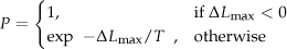
The SA algorithm is commonly used for solving combinatorial optimization problems. It starts from an initial basic solution $x_0$ and randomly generates a neighbour solution $x^{\prime }$ from its neighbourhood. $x^{\prime }$ is accepted as a new basic solution with probability P, which is calculated as

$P=(\begin{array}{cc}\mathrm{1,}& \text{if}\hspace{0.17em}\hspace{0.17em}\hspace{0.17em}\mathrm{\Delta }{L}_{\max }\text{<0}\\ \exp \{-\mathrm{\Delta }{L}_{\max }/T\}\mathrm{,}& \text{otherwise}\end{array}$

where $\mathrm{\Delta }{L}_{\max }=L_{\max }(x^{\prime })-L_{\max }(x_0)$ is the difference in objective value between the two solutions, and T is the temperature which decreases with iterations. The searching process keeps generating a neighbour solution and accepting it with the above probability until some stopping criterion is met. The framework of the standard SA algorithm can be described as follows.

Step 1. Produce an initial solution $x_0$ . Set $x^{\ast }=x_0$ .

Step 2. For $iter=\mathrm{1,2,}\dots \mathrm{,}{I}_{\max }$

• (2.1)

  Randomly generate a neighbour solution $x^{\prime }$ from the neighbourhood of $x_0$ .

• (2.2)

  If $L_{\max }(x^{\prime })<L_{\max }(x^{\ast })$ , set $x^{\ast }=x^{\prime }$ .

• (2.3)

  Set $x_0=x^{\prime }$ with probability $P=\min \{\mathrm{1,}\exp \{(L_{\max }(x_0)-L_{\max }(x^{\prime }))/T\}\}$ .

• (2.4)

  Reduce the temperature by setting $T:=T\times \lambda$ , where $\lambda \in (\mathrm{0,1})$ is the cooling rate.

Step 3. Return x^∗.

3.2. Constraint Propagation (CP)

In this part, we will introduce the basic application of CP theory to job shop scheduling.

We use $\mathcal{P}=(O\mathrm{,}C\mathrm{,}D\mathrm{,}P)$ to denote a specific JSSP instance. As introduced above, $O=\{\mathrm{1,}\dots \mathrm{,}n\times m\}$ is the set of operations; C is the set of conjunctive arcs and $(i\mathrm{,}j)\in C$ indicates operation i must be processed before operation j; D is the set of disjunctive arcs and $(i\mathrm{,}j)\in D$ indicates operation i cannot overlap with operation j in processing; $P=\{p_i|i\in O\}$ is the set of operation processing times.

In order to apply CP to JSSP, it is required to first give an upper bound $UB$ for the optimal $L_{\max }$ of the instance. Therefore, if we use ${\delta }_i$ to denote the feasible domain of starting times of each operation $i\in O$ , we must have ${\delta }_i\subseteq [\mathrm{0,}UB+d_i-p_i]$ . Normally, the tighter the upper bound, the more information will be derived by CP.

The earliest starting time and the latest starting time of operation i are respectively defined as $es{t}_i=\min {\delta }_i$ , $ls{t}_i=\max {\delta }_i$ . Thus, ${\delta }_i$ can also be expressed as ${\delta }_i=[es{t}_i\mathrm{,}ls{t}_i]=\{es{t}_i\mathrm{,}es{t}_i+\mathrm{1,}\dots \mathrm{,}ls{t}_i-\mathrm{1,}ls{t}_i\}$ . Meanwhile, we define the earliest completion time and the latest completion time of operation i respectively as $ec{t}_i=es{t}_i+p_i$ and $lc{t}_i=ls{t}_i+p_i$ .

For a subset of operations $A\subseteq O$ (which need to be processed on the same machine), we define the following functions: $P(A)={\displaystyle {\sum }_{i\in A}}{p}_i$ , $ES{T}_{\min }(A)={{\displaystyle \min }}_{i\in A}es{t}_i$ and $LC{T}_{\max }(A)={{\displaystyle \max }}_{i\in A}lc{t}_i$ .

In the following, some of the most important principles for applying CP to JSSP are presented [9].

Theorem 1 (Conjunctive consistency test) If $i\mathrm{,}j\in O$ and $(i\mathrm{,}j)\in C$ , then the following domain reduction rule is effective:

$\begin{array}{l}es{t}_j:=\max \{es{t}_j\mathrm{,}es{t}_i+p_i\}\mathrm{,}\hfill \\ ls{t}_i:=\min \{ls{t}_i\mathrm{,}ls{t}_j-p_i\}\mathrm{.}\hfill \\ \hfill \end{array}$

Clearly, the time complexity of revising the earliest/latest starting times is $O((nm{)}^2)$ .

Theorem 2 (Input/output sequence consistency test) Assume $A⊊O$ and $i\notin A$ , if the following “input condition” is satisfied:

$\underset{u\in A\mathrm{,}v\in A\cup \{i\}\mathrm{,}u\ne v}{{\displaystyle \max }}\{lc{t}_v-es{t}_u\}<P(A\cup \{i\}),$

then operation i must be completed before every operation in A. Similarly, if the following “output condition” is satisfied:

$\underset{u\in A\cup \{i\}\mathrm{,}v\in A\mathrm{,}u\ne v}{{\displaystyle \max }}\{lc{t}_v-es{t}_u\}<P(A\cup \{i\})\mathrm{,}$

then operation i must be processed after every operation in A.

When $\left|A\right|=1$ , the above theorem can be stated as: if $i\ne j$ and $lc{t}_j-es{t}_i<p_i+p_j$ , then the disjunctive arc direction $j\to i$ can be fixed. Such a “pair-wise test” can be performed in $O((nm{)}^2)$ time.

Theorem 3 (Output domain consistency test) If there exist $A⊊O$ and $i\notin A$ which satisfy the output condition, then the earliest starting time of operationi can be adjusted as

$es{t}_i:=\max \{es{t}_i\mathrm{,}ES{T}_{\min }(A)+P(A)\}\mathrm{.}$

Naturally, a dual conclusion exists for describing the input condition.

Theorem 4 (Input/output negation sequence consistency test)Assume $A⊊O$ and $i\notin A$ , if the following “input negation condition” is satisfied:

$LC{T}_{\max }(A)-es{t}_i<P(A\cup \{i\})\mathrm{,}$

then operation i cannot be completed before every operation in A. Similarly, if the following “output negation condition” is satisfied:

$lc{t}_i-ES{T}_{\min }(A)<P(A\cup \{i\})\mathrm{,}$

then operation i cannot be processed after every operation in A.

Theorem 5 (Input negation domain consistency test) If there exist $A⊊O$ and $i\notin A$ which satisfy the input negation condition, then the earliest starting time of operation i can be adjusted as

$es{t}_i:=\max \left\{es{t}_i\mathrm{,}\underset{u\in A}{{\displaystyle \min }}\{ec{t}_u\}\right\}\mathrm{.}$

Naturally, a dual conclusion exists for describing the output negation condition.

Besides the listed theorems, there are some others, such as the input-or-output consistency test. In the subsequent part of the paper, the application of CP to JSSP is regarded as an independent module, the procedure of which can be found in [14].

4. The algorithm

4.1. The decomposition method

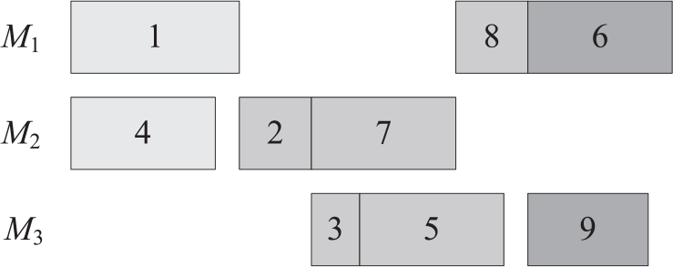
The decomposition scheme used in this paper can be intuitively illustrated using a disjunctive graph like Figure 1, in which nine operations of three jobs are to be processed on three machines. According to the conjunctive arcs, operations 1-3 belong to job 1, operations 4-6 belong to job 2 and operations 7-9 belong to job 3. According to the disjunctive arcs, operations 1, 6 and 8 are to be processed by machine 1, operations 2, 4 and 7 are to be processed by machine 2, and operations 3, 5 and 9 are to be processed by machine 3. The dividing curves representing a decomposition policy divide the operation set into three sequential subsets: I, II and III, each of which corresponds to a subproblem.

Figure 1.

An illustration of the decomposition method

To be precise, the decomposition method has the following properties: (1) If the original operation set is divided into p subsets ${\left\{O_l\right\}}_{l=1}^p$ , then ${\displaystyle {\cup }_{l=1}^p}{O}_l=O$ , and $\forall l\ne l^{\prime }$ , $O_l\cap O_{l^{\prime }}=\varnothing$ ; (2) For any two operations i and j, if $\left(i\mathrm{,}j\right)\in C$ and $i\in O_{l_i}$ , $j\in O_{l_j}$ , then $l_i\le l_j$ .

4.2. Using CP as a preprocessor for JSSP

From Section 3.2, we see that CP can derive the correct direction of some disjunctive arcs by alternating sequence consistency tests and domain consistency tests. The following algorithm is designed by combining CP with local search in an iterative fashion so that a tight upper bound can be used to orient a sufficient number of disjunctive arcs.

Input: The problem instance $\mathcal{P}=(O\mathrm{,}C\mathrm{,}D\mathrm{,}P)$ .

Step 1. Construct the initial solution $S_1$ based on the EDD (earliest due date) dispatching rule. Let $UB=L_{\max }(S_1)$ , where $L_{\max }(\cdot )$ denotes the objective value of a solution. Let the initial set of directed disjunctive arcs $\widehat{D}=\varnothing$ and $k=1$ .

Step 2. Perform a stochastic local search starting from $S_k$ (employing w iterations) in order to find a new best-so-far solution $S^{\ast }$ and update the upper bound $UB=L_{\max }(S^{\ast })$ . If no improvement is found within the w iterations, then output $\widehat{D}$ .

Step 3. Add a set of new constraints “ $\forall i\in O$ , $lc{t}_i:=\min \{lc{t}_i\mathrm{,}UB-\mathrm{\Delta }\}$ ” and then call the CP module to derive as much information as possible. The disjunctive arc directions newly obtained in this step are denoted as $D^{\prime }$ . If ${\delta }_i=\varnothing$ for some operation or $C\cup \widehat{D}\cup D^{\prime }$ contains cycles, output $\widehat{D}$ . Otherwise, let $\widehat{D}:=\widehat{D}\cup D^{\prime }$ and $k:=k+1$ .

Step 4. Taking $C\cup \widehat{D}$ as the precedence constraints, construct a new solution $S_k$ based on the EDD rule. If $L_{\max }(S_k)<UB$ , let $UB=L_{\max }(S_k)$ . Go back to Step 2.

The above algorithm can be used as a preprocessor which is applied to a JSSP instance before we start to solve it. The two parameters involved in this procedure are w (the number of iterations in each run of local search) and Δ (the step size when lowering the upper bound). The resolved disjunctive arcs $\widehat{D}$ will be used to determine a decomposition policy for the JSSP instance.

4.3. Finding a decomposition policy

A decomposition policy determines the structures of all the subproblems at a time and thus it directly affects the subsequent optimization process. In this paper, a simulated annealing (SA) approach is designed to search for a satisfactory decomposition policy based on the previously derived disjunctive arc directions.

SA searches among all possible decomposition policies and outputs a promising policy, which divides the operation set into p successive subsets by satisfying the maximum number of derived disjunctive arcs. The input parameters include the desired number of operations in each produced subset, i.e., ${\left\{{\alpha }_l\right\}}_{l=1}^p$ .

A directed disjunctive arc $(i\mathrm{,}j)$ is “satisfied” if the subset containing operation i is not preceded by the subset containing operation j. With respect to the previous example (see Figure 2 here), if the disjunctive arcs $(\mathrm{1,8})$ and $(\mathrm{6,8})$ have been oriented by CP, then the illustrated decomposition policy satisfies $(\mathrm{1,8})$ (because operation 1 is in subset I and operation 8 is in subset II), but does not satisfy $(\mathrm{6,8})$ (because subset II, which includes operation 8, precedes subset III which includes operation 6). To be precise, suppose $\left(i\mathrm{,}j\right)\in \widehat{D}$ and the considered decomposition policy (dividing the original operation set into p successive subsets ${\left\{O_l\right\}}_{l=1}^p$ ) indicates $i\in O_{l_i}$ , $j\in O_{l_j}$ , then $(i\mathrm{,}j)$ is satisfied only if $l_i\le l_j$ .

Figure 2.

An illustration of satisfied and dissatisfied arcs

4.3.1. Encoding

A matrix $B=[b_{j\mathrm{,}l}{]}_{n\times p}$ is used to encode a solution, where the element $b_{j\mathrm{,}l}$ denotes the number of operations that belong to job j and have been assigned to subset $O_l$ . According to this definition, B has to satisfy:

$\begin{array}{ll}{\displaystyle \sum _{l=1}^p}{b}_{j\mathrm{,}l}=m\mathrm{,}\hfill & j=\mathrm{1,}\dots \mathrm{,}n\mathrm{,}\hfill \\ {\displaystyle \sum _{j=1}^n}{b}_{j\mathrm{,}l}={\alpha }_l\mathrm{,}\hfill & l=\mathrm{1,}\dots \mathrm{,}p\mathrm{.}\hfill \end{array}$

In the above equations, m is exactly the number of operations included by each job. Besides, since the operations of each job are decomposed according to their technological order, a matrix in the form of B is sufficient for encoding a solution in the SA.

For example, the decomposition policy shown in Figure 2 should be encoded as

$B_0=\left[\begin{array}{ccc}1& 2& 0\\ 1& 1& 1\\ 0& 2& 1\end{array}\right]\mathrm{,}$

where the first row means the 1st operation of job 1 is assigned to the subset I, the next two operations of job 1 are assigned to subset II, while no operation of job 1 is assigned to subset III.

4.3.2. Initialization

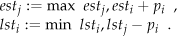
A heuristic rule similar to EDD is used to produce the initial solution. For each operation i in O, we define the modified due date $h_i$ as:

$h_i=\{\begin{array}{ll}{d}_i\mathrm{,}\hfill & \text{if}\hspace{0.17em}\hspace{0.17em}\hspace{0.17em}\text{{j:(i,j)}\in \mathrm{C}\cup \widehat{D}\text{}=}\varnothing \\ \underset{(i\mathrm{,}j)\in C\cup \widehat{D}}{{\displaystyle \min }}\{h_j-p_j\}\mathrm{,}\hfill & \text{otherwise}\end{array}$

where $d_i$ is the due date of the job to which operation i belongs. Just like $d_i$ , the newly defined $h_i$ also describes the urgency level of operation i, but in a more strict manner than the original due date.

Then, all the operations are sorted in a non-decreasing order of $h_i$ , yielding an operation sequence $[i_1\mathrm{,}{i}_2\mathrm{,}\dots \mathrm{,}{i}_{nm}]$ . After that, the p subsets are successively assigned with operations in the order specified by this sequence.

According to the encoding scheme, the value of $b_{j\mathrm{,}l}$ (the number of job j's operations that have been assigned to subset $O_l$ ) can now be acquired, and thus, the encoding matrix $B^{(1)}$ for this initial decomposition policy is obtained.

4.3.3. New solution generation

In order to generate a new solution from the current solution, the algorithm randomly selects an element $b_{j\mathrm{,}l}$ from B and sets $b_{j\mathrm{,}l}\leftarrow b_{j\mathrm{,}l}+\xi$ where ξ is a two-value random variable in $\left\{+\mathrm{1,}-1\right\}$ with probability $\{\frac{1}{2}\mathrm{,}\frac{1}{2}\}$ . For keeping the row sum and the column sum of B constant, the algorithm randomly selects another three elements $b_{j\mathrm{,}{l}^{\prime }}\mathrm{,}{b}_{j^{\prime }\mathrm{,}l}$ and $b_{j^{\prime }\mathrm{,}{l}^{\prime }}$ ( $j^{\prime }\ne j\mathrm{,}{l}^{\prime }\ne l$ ) from B and sets $b_{j\mathrm{,}{l}^{\prime }}:=b_{j\mathrm{,}{l}^{\prime }}-\xi$ , $b_{j^{\prime }\mathrm{,}l}:=b_{j^{\prime }\mathrm{,}l}-\xi$ and $b_{i^{\prime }\mathrm{,}{j}^{\prime }}:=b_{j^{\prime }\mathrm{,}{l}^{\prime }}+\xi$ . Notably, it must be ensured that the resulting matrix elements satisfy $b_{j\mathrm{,}l}\ge \mathrm{0,}\forall j\mathrm{,}l$ .

4.3.4. Evaluation

The number of satisfied disjunctive arcs is adopted as the objective function of SA in this stage. Therefore, the evaluation of a solution is formally described as

$f(B)={\displaystyle \sum _{(i\mathrm{,}j)\in \widehat{D}}}{z}_{(i\mathrm{,}j)}\mathrm{,}$

where $z_{(i\mathrm{,}j)}=1$ if the derived arc $(i\mathrm{,}j)$ is satisfied and $z_{(i\mathrm{,}j)}=0$ otherwise.

For example, the decomposition policy shown in Figure 2 has an objective value of

$f(B_0)=z_{(\mathrm{1,8})}+z_{(\mathrm{4,2})}+z_{(\mathrm{3,5})}+z_{(\mathrm{6,8})}+z_{(\mathrm{3,9})}=\mathrm{4,}$

because the directed disjunctive arcs are all satisfied except $(\mathrm{6,8})$ .

4.4. Solving each subproblem

In this paper, the process of solving each subproblem is equivalent to optimizing the sequence of the operations involved in this subproblem ( $O_l$ ). To this end, a simulated annealing algorithm is designed. The main steps to solve the l -th subproblem are described as follows.

4.4.1. Encoding

The encoding scheme is based on operation priority lists. A solution relates each machine with a priority list of the operations (from $O_l$ ) to be processed on this machine. Note that after the decoding process, the actual processing order of the operations in the final feasible schedule may differ from the priority lists.

4.4.2. Initialization

The initial solution is provided by the EDD dispatching rule, where the due date of each operation is taken as $h_i$ .

4.4.3. New solution generation

In order to generate a new solution from the current solution, we must first identify a machine and then somehow alter the operation list related with the selected machine. Hence, machine selection is a key step in this process. We hope to select the machines which are scheduled not very well and therefore have relatively larger room for further improvement.

To achieve this aim, we define an index ${\mathrm{\Psi }}_k$ for each machine k to evaluate the scheduling efficiency of this machine:

${\mathrm{\Psi }}_k={\displaystyle \sum _{i\in O_{kl}}}{\left(c_i-h_i\right)}^{+}\mathrm{,}$

where $O_{kl}$ is the set of operations to be processed by machine k in $O_l$ ; $c_i$ is the completion time of operation i in the current schedule; $x^{+}=\max \{x\mathrm{,0}\}$ . ${\mathrm{\Psi }}_k$ reflects the scheduling performance of machine k, and a larger value of ${\mathrm{\Psi }}_k$ suggests machine k is currently scheduled less satisfactorily. Therefore, if we focus more of the subsequent optimization efforts on those machines with higher Ψ values, it is more likely to obtain improvement. So the proportional method (a.k.a. roulette wheel selection) is adopted here for the selection of a machine, i.e., machine k is selected with probability $Pro{b}_k={\mathrm{\Psi }}_k/{\displaystyle {\sum }_{k=1}^m}{\mathrm{\Psi }}_k$ .

Finally, the “SWAP” operator is used to exchange the positions of two randomly chosen operations in the selected machine's priority list, and then a new solution is produced.

4.4.4. Evaluation

The decoding process iteratively schedules the ready operations in the current subproblem according to their priority order indicated by the solution and as early as possible, on the basis of the partial schedule obtained in the previous subproblems $O_1\mathrm{,}\dots \mathrm{,}{O}_{l-1}$ (a data structure similar to the Gantt chart is used to record the partial schedules obtained in previous subproblems).

Taking the instance shown in Figure 2 as an example, we can see the incremental process of solving each subproblem. After subproblem 1 is solved, the positions of operations 1 and 4 (light grey) should be fixed, which form the basis for solving subproblem 2. After subproblem 2 is solved, the positions of operations 8, 2, 7, 3 and 5 (medium grey) should be fixed, which, together with the previously fixed operations 1 and 4, form the basis for solving subproblem 3. Once subproblem 3 has been solved, the positions of operations 6 and 9 (dark grey) should be fixed. Now, we could obtain a complete solution to the original problem, as shown in Figure 3.

Figure 3.

Solving the three subproblems successively

The evaluation of a solution is based on the local objective function defined as

$L_{\max }^{\text{local}}=\underset{j=1}{\overset{n}{{\displaystyle \max }}}\{c_{{\omega }_l(j)}-h_{{\omega }_l(j)}\}\mathrm{,}$

where ${\omega }_l(j)$ denotes the last operation in the technological route of job j that belongs to the current subproblem $O_l$ . Taking the case described in Figure 3 as an example, when we are solving subproblem 2, the local objective function should be evaluated based on operations 3, 5 and 8, that is, ${\omega }_2(1)=3$ , ${\omega }_2(2)=5$ , ${\omega }_2(3)=8$ .

5. Computational experiments

In this section, some JSSP benchmark instances from the OR-Library [6] are used to evaluate the performance of DOASA. Since this research is aimed at large-scale problems, only the instances that include no less than 300 operations are tested. These 27 instances belong to the LA, ABZ, SWV and YN classes. Moreover, in order to adapt the instances for the $L_{\max }$ objective function considered here, the due date of each job is set based on its total processing time as $d_j=f\times {\displaystyle {\sum }_{i\in J_j}}{p}_i$ , where ${\displaystyle {\sum }_{i\in J_j}}{p}_i$ is the sum of processing times of all the operations that constitute job j, and $f\in \{\mathrm{1.3,1.4,1.5}\}$ is the due date tightness factor.

In the computational experiments, the parameters for SA are set as: the initial acceptance probability $p_{\mathrm{r}}=0.8$ ; the temperature reduction ratio $\lambda =0.95$ ; the number of inner iterations (number of samples obtained at each temperature) $I_{\mathrm{i}}=20$ ; the number of outer iterations (number of temperature stages) $I_{\mathrm{o}}=50$ . The parameters for the CP-based preprocessor is set as: the local search iteration number $w=100$ ; the step size for locating upper bound $\mathrm{\Delta }=3$ . Meanwhile, the number of subproblems for each instance is fixed according to some preliminary computational results: for the instances with 500 operations (SWV11–SWV20), $p=6$ is adopted; for the remaining instances with 300 or 400 operations, $p=4$ is adopted. Once p is fixed, the number of operations in each subproblem is

${\alpha }_l=\{\begin{array}{ll}\lfloor \frac{\left|O\right|}{p+1}\rfloor \mathrm{,}\hfill & l=\mathrm{1,}\dots \mathrm{,}p-1\hfill \\ \left|O\right|-\left(p-1\right)\times \lfloor \frac{\left|O\right|}{p+1}\rfloor \mathrm{,}\hfill & l=p\hfill \end{array}$

The last subproblem contains more operations in order to facilitate the final adjustment of the schedule for improving the objective value.

In order to examine the effectiveness of the presented approach, DOASA is compared with the following methods:

• The genetic algorithm (GA) applying operation-based encoding scheme and heuristic initialization;

• The fast TS/SA hybrid algorithm which combines the advantages of tabu search and simulated annealing [24];

In the GA, the initial population is generated by applying various effective dispatching rules, including SPT, EDD, MDD, etc. [13]. The parameters of GA are set as: the population size is 100, the maximum generation number is 500 (or determined by the exogenous limit on computational time), the crossover probability is 0.8 and the mutation probability is 0.1. The parameters of TS/SA are determined according to the original literature [24].

All the algorithms are implemented in Visual C++ 7 and tested on an Intel Core i5-750 / 3GB RAM / Windows 7 platform. To make the comparison meaningful, we keep the running time of each algorithm identical. In each trial, we run DOASA first and record its computational time as $CT$ , and then run GA and TS/SA under the time limit of $CT$ (which controls the realized number of iterations for each algorithm).

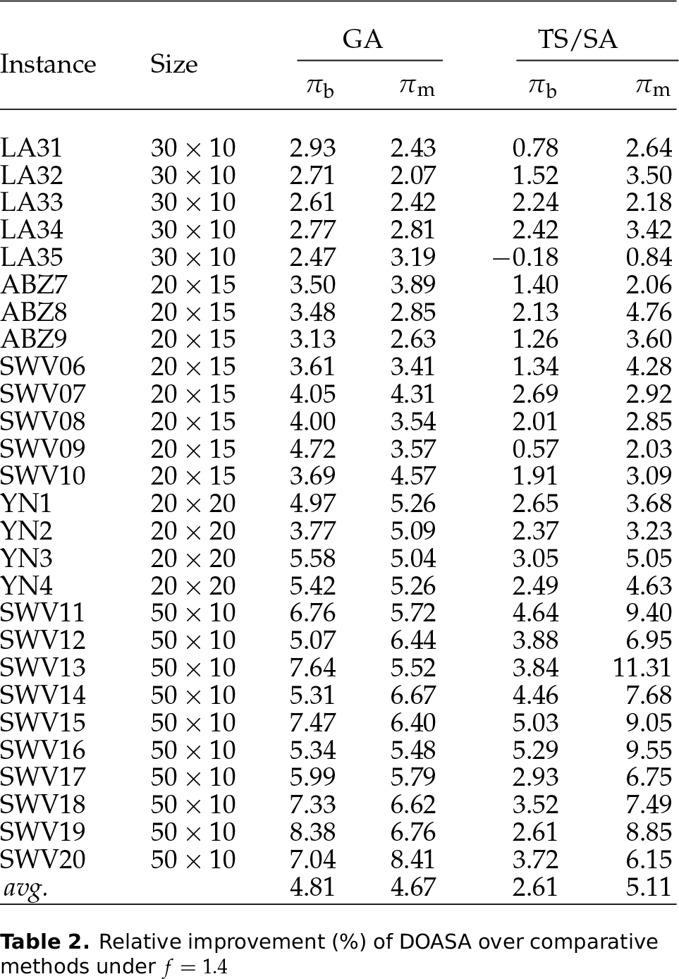
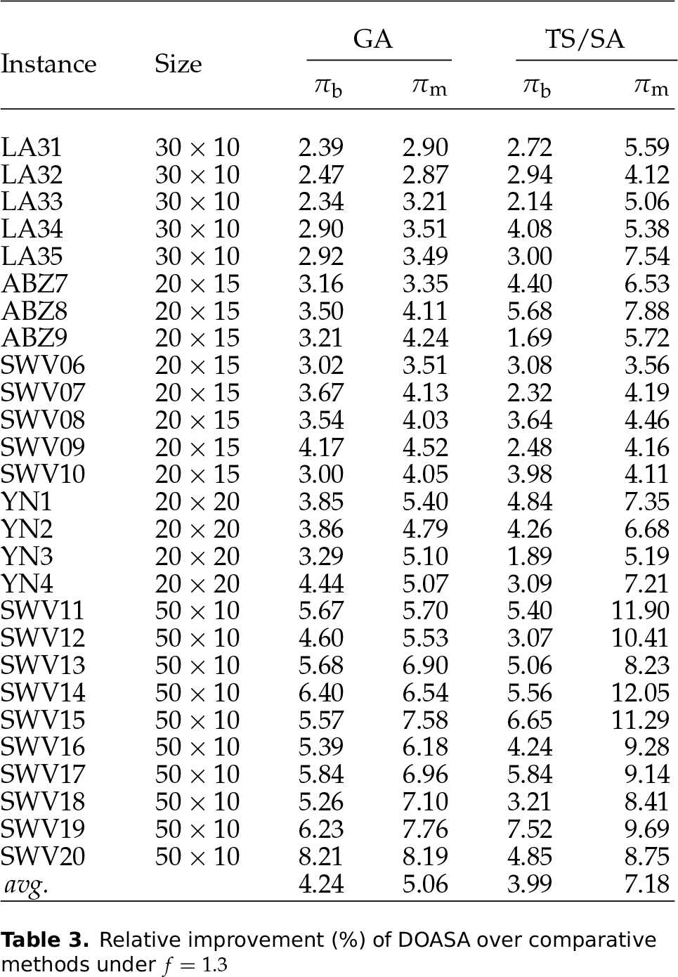
Table 1 presents the results for wide due date settings ( $f=1.5$ ), Table 2 presents the results for moderate due date settings ( $f=1.4$ ), and Table 3 presents the results for tight due date settings ( $f=1.3$ ). In the tables, the first two columns list the instance names and their sizes in the format of $n\times m$ . For each instance, all the algorithms are allowed to run 10 independent times. Since absolute objective values are unimportant for comparison purposes, the focus here is put on relative values. ${\pi }_{\mathrm{b}}$ is used to characterize the improvement (in percentage) of the best solution obtained by DOASA during the 10 runs over the best solution by the comparative method. Formally, we define

${\pi }_{\mathrm{b}}(a\mathrm{,}\mathcal{I})=\frac{L_{\max }^{\text{best}}(a\mathrm{,}\mathcal{I})-L_{\max }^{\text{best}}(\text{DOASA}\mathrm{,}\mathcal{I})}{L_{\max }^{\text{best}}(\text{DOASA}\mathrm{,}\mathcal{I})}\mathrm{,}$

where $L_{\max }^{\text{best}}(a\mathrm{,}\mathcal{I})$ is the best objective value for instance $\mathcal{I}$ obtained by the algorithm a ( $a\in \{GA\mathrm{,}TS/SA\mathrm{,}DOASA\}$ ) in the 10 runs. Defined similarly, ${\pi }_{\mathrm{m}}$ denotes the percentage improvement of the mean objective value obtained by DOASA during the 10 runs over the mean objective value by the comparative method (detailed formula omitted here). The maximum lateness $L_{\max }$ remains positive even under $f=1.5$ so that the relative values ( ${\pi }_{\mathrm{b}}$ , ${\pi }_{\mathrm{m}}$ ) are meaningful and comparable.

Table 1.

Relative improvement (%) of DOASA over comparative methods under $f=1.5$

Instance	Size	GA		TS/SA
		πb	πm	πb	πm
LA31	30 × 10	2.13	1.99	0.65	1.91
LA32	30 × 10	1.80	1.92	1.40	2.73
LA33	30 × 10	2.27	2.16	1.84	2.16
LA34	30 × 10	2.12	2.33	1.99	2.71
LA35	30 × 10	2.17	2.44	0.22	0.56
ABZ7	20 × 15	2.31	2.93	1.36	1.82
ABZ8	20 × 15	2.35	2.96	1.94	3.96
ABZ9	20 × 15	2.06	2.41	1.12	3.13
SWV06	20 × 15	2.46	2.73	1.14	3.50
SWV07	20 × 15	2.87	3.66	2.08	2.06
SWV08	20 × 15	3.22	3.06	1.74	2.34
SWV09	20 × 15	3.58	3.76	−0.51	1.73
SWV10	20 × 15	3.07	4.04	1.43	2.54
YN1	20 × 20	3.76	3.63	2.08	3.16
YN2	20 × 20	3.43	4.18	1.74	2.66
YN3	20 × 20	4.15	3.73	2.66	4.01
YN4	20 × 20	4.23	3.79	2.53	3.29
SWV11	50 × 10	4.14	4.67	3.97	6.62
SWV12	50 × 10	3.91	5.14	3.19	5.84
SWV13	50 × 10	4.46	4.93	3.62	9.38
SWV14	50 × 10	4.98	5.26	3.88	6.21
SWV15	50 × 10	5.29	5.29	4.35	7.92
SWV16	50 × 10	3.80	5.06	4.48	8.24
SWV17	50 × 10	5.20	5.82	2.59	5.67
SWV18	50 × 10	5.13	5.65	3.17	6.46
SWV19	50 × 10	5.57	6.68	2.42	6.34
SWV20	50 × 10	5.45	6.29	3.55	5.76
avg.		3.55	3.94	2.25	4.17

Table 2.

Relative improvement (%) of DOASA over comparative methods under $f=1.4$

Instance	Size	GA		TS/SA
		πb	πm	πb	πm
LA31	30 × 10	2.93	2.43	0.78	2.64
LA32	30 × 10	2.71	2.07	1.52	3.50
LA33	30 × 10	2.61	2.42	2.24	2.18
LA34	30 × 10	2.77	2.81	2.42	3.42
LA35	30 × 10	2.47	3.19	−0.18	0.84
ABZ7	20 × 15	3.50	3.89	1.40	2.06
ABZ8	20 × 15	3.48	2.85	2.13	4.76
ABZ9	20 × 15	3.13	2.63	1.26	3.60
SWV06	20 × 15	3.61	3.41	1.34	4.28
SWV07	20 × 15	4.05	4.31	2.69	2.92
SWV08	20 × 15	4.00	3.54	2.01	2.85
SWV09	20 × 15	4.72	3.57	0.57	2.03
SWV10	20 × 15	3.69	4.57	1.91	3.09
YN1	20 × 20	4.97	5.26	2.65	3.68
YN2	20 × 20	3.77	5.09	2.37	3.23
YN3	20 × 20	5.58	5.04	3.05	5.05
YN4	20 × 20	5.42	5.26	2.49	4.63
SWV11	50 × 10	6.76	5.72	4.64	9.40
SWV12	50 × 10	5.07	6.44	3.88	6.95
SWV13	50 × 10	7.64	5.52	3.84	11.31
SWV14	50 × 10	5.31	6.67	4.46	7.68
SWV15	50 × 10	7.47	6.40	5.03	9.05
SWV16	50 × 10	5.34	5.48	5.29	9.55
SWV17	50 × 10	5.99	5.79	2.93	6.75
SWV18	50 × 10	7.33	6.62	3.52	7.49
SWV19	50 × 10	8.38	6.76	2.61	8.85
SWV20	50 × 10	7.04	8.41	3.72	6.15
avg.		4.81	4.67	2.61	5.11

Table 3.

Relative improvement (%) of DOASA over comparative methods under $f=1.3$

Instance	Size	GA		TS/SA
		πb	πm	πb	πb
LA31	30 × 10	2.39	2.90	2.72	5.59
LA32	30 × 10	2.47	2.87	2.94	4.12
LA33	30 × 10	2.34	3.21	2.14	5.06
LA34	30 × 10	2.90	3.51	4.08	5.38
LA35	30 × 10	2.92	3.49	3.00	7.54
ABZ7	20 × 15	3.16	3.35	4.40	6.53
ABZ8	20 × 15	3.50	4.11	5.68	7.88
ABZ9	20 × 15	3.21	4.24	1.69	5.72
SWV06	20 × 15	3.02	3.51	3.08	3.56
SWV07	20 × 15	3.67	4.13	2.32	4.19
SWV08	20 × 15	3.54	4.03	3.64	4.46
SWV09	20 × 15	4.17	4.52	2.48	4.16
SWV10	20 × 15	3.00	4.05	3.98	4.11
YN1	20 × 20	3.85	5.40	4.84	7.35
YN2	20 × 20	3.86	4.79	4.26	6.68
YN3	20 × 20	3.29	5.10	1.89	5.19
YN4	20 × 20	4.44	5.07	3.09	7.21
SWV11	50 × 10	5.67	5.70	5.40	11.90
SWV12	50 × 10	4.60	5.53	3.07	10.41
SWV13	50 × 10	5.68	6.90	5.06	8.23
SWV14	50 × 10	6.40	6.54	5.56	12.05
SWV15	50 × 10	5.57	7.58	6.65	11.29
SWV16	50 × 10	5.39	6.18	4.24	9.28
SWV17	50 × 10	5.84	6.96	5.84	9.14
SWV18	50 × 10	5.26	7.10	3.21	8.41
SWV19	50 × 10	6.23	7.76	7.52	9.69
SWV20	50 × 10	8.21	8.19	4.85	8.75
avg.		4.24	5.06	3.99	7.18

The results in Tables 1–3 reveal the effectiveness of DOASA. The following remarks can be made regarding the algorithm's performance.

1. At each due date level, the superiority of DOASA over the comparative methods is more significant for the larger instances (SWV11–SWV20 with $p=6$ ) than for the smaller instances (with $p=4$ ). This can be interpreted as evidence that decomposing a large JSSP instance into smaller subproblems will make the search process more efficient during optimization.

2. It is observed that for most instances, ${\pi }_{\mathrm{m}}>{\pi }_{\mathrm{b}}$ holds, which means the improvement on mean objective value is usually greater than the improvement on best objective value. So it is reasonable to conclude that the stability of DOASA in different executions is considerably stronger than the comparative algorithms. The robustness is an advantage brought by the decomposition-based optimization framework which builds the final schedule in an incremental way.

3. By comparing the average ${\pi }_{}b$ of GA and TS/SA, we may find that TS/SA performs better than GA in terms of the best solution quality. This can be explained by the fact that the combination of TS and SA significantly enhances the exploitation ability of the search algorithm. Then, if we compare the average ${\pi }_{}m$ of GA and TS/SA, we find that GA outperforms TS/SA in terms of the mean solution quality. Therefore, in spite of its weakness in intensified search, GA performs more stably in different runs due to its population-based searching behaviour.

4. By comparing the three tables, it is apparent that the relative improvement of DOASA over the comparative algorithms is larger in the case of a tighter due date (i.e., smaller f). Such a difference in due date robustness also reflects the effectiveness of the decomposition procedure based on constraint propagation. When the due dates are tighter (i.e., $UB+d_i-p_i$ is smaller), more disjunctive arc directions can be derived by constraint propagation, which helps to generate a more useful and reliable decomposition policy.

The computational time consumed by DOASA when solving the four representative instances is shown in Figure 4. The due date tightness affects the process of constraint propagation and operation decomposition, so the time needed for handling tight due dates is higher than for wide due dates.

Figure 4.

The computational time consumed by DOASA

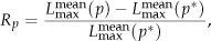
To test the impact of subproblem number (p) on the final solution quality, the results obtained by DOASA under different p values for two selected instances (SWV06 and SWV11) are recorded and shown as relative percentage values in Figure 5. In this figure, we define

Figure 5.

The impact of p on solution quality

$R_p=\frac{L_{\max }^{mean}(p)-L_{\max }^{mean}(p^{\ast })}{L_{\max }^{mean}(p^{\ast })}\mathrm{,}$

where $L_{\max }^{mean}(p)$ denotes the obtained mean objective value in 10 runs when the subproblem number is set as p, and $p^{\ast }=\arg {{\displaystyle \min }}_{p\in \mathcal{P}}{L}_{\max }^{mean}(p)$ is the optimal subproblem number within the considered range ( $\mathcal{P}$ ) of possible p values.

Figure 5 suggests the subproblem number in DOASA can affect the solution quality to a noticeable extent. We have $p^{\ast }=4$ for the instance SWV06 and $p^{\ast }=6$ for the instance SWV11. When the actual subproblem number is far less than $p^{\ast }$ , the optimization result is much poorer because the benefit of decomposition has not been fully utilized. On the other extreme, if the adopted subproblem number is unduly large, the solution quality also deteriorates because the additional preferential order imposed by the decomposition procedure can reduce the potential search space, thus limiting the subsequent optimization process for each subproblem.

6. Conclusion

A decomposition-based optimization algorithm is proposed in this paper for large-sized job shop scheduling problems with the maximum lateness criterion. The theory of constraint propagation is utilized as a preprocessor for the pending problem instance so that a number of disjunctive arcs can be correctly oriented. Simulated annealing is adopted as the main framework in the two optimization procedures, i.e., the search for a promising decomposition policy and the solving of each subproblem. Experiments have been carried out for adapted JSSP benchmark instances. The performance of the proposed algorithm surpasses the competing methods (under the same computational time limit), especially for larger instances and under tighter due date settings. The results verify the effectiveness and efficiency of both the decomposition procedure and the subproblem solution procedure. In the future research, parallel computing (e.g., based on GPU) techniques may be considered as a method for accelerating the execution of the proposed algorithm. In this way, the subproblems can be solved in parallel once they have been determined by the decomposition procedure, which will shorten the running time considerably.