
Abstract
In this article, a neural network corrector is proposed to correct the image shift, yielding the degradation of three-dimensional image reconstruction, for each slice captured by cone-beam computed tomography simulator. There are 3 degrees of freedom in tube module of simulator; the central point of tube module should be aligned with the central point of detector module to guarantee the accurate image projection. However, the mechanism manufacturing and assembling tolerance will let the above aim cannot be met. Here, a standard kit is made to measure the image shift by 1° step from −10° to 10°. The measure data will be the input training data of proposed neural network corrector, and the corrected translation position will be the output of neural network corrector. The Levenberg–Marquardt learning algorithm adjusts the connected weights and biases of the neural network using a supervised gradient descent method, such that the defined error function can be minimized. To avoid the problem of overfitting and improve the generalized ability of the neural network, Bayesian regularization is added to the Levenberg–Marquardt learning algorithm. After the training of neural network corrector, the different target position commands are fed into the neural network corrector. Then, the corrected data from neural network corrector are fed to be the new position command to verify the image correction performance. Moreover, a phantom kit is made to check the corrected performance of the neural network corrector. Finally, the experimental results verify that the image shift can be reduced by the neural network corrector.
Keywords
Introduction
Traditionally, X-ray computed tomography (X-CT) was used to perform the operation of tumor resection and tooth implantation. X-CT system was also called fan-beam system, and the rotating frame was made up of X-ray source and one-dimensional (1D) linear detector, as shown in Figure 1(a). The frame was rotated a circle to obtain 1D images from 1D linear detector and reconstructed to two-dimensional (2D) images. Then, the 2D images were used to execute three-dimensional (3D) image reconstruction. 1

(a) X-CT, (b) MDCT, and (c) 16 rows image detector.
The normal mode of X-CT was multi-detector row computed tomography (MDCT), which used multi-slice method to obtain the 2D images by scanning the patient, as shown in Figure 1(b). X-ray source and detector were rotated continuously, and the table was moved linearly. This mode can obtain multiple images and simultaneously improve the scanning speed. Moreover, the image detector had been increased to 16 rows or 128 rows, as shown in Figure 1(c), such that all images could be obtained more quickly. 2
However, the efficiency of X-CT was not good enough, resulting in longer scan time, higher patient radiation dose, and longer primary reconstruction time. So, cone-beam computed tomography (CBCT) was proposed to improve the drawback of X-CT. CBCT was a modification of X-CT. The difference between these two modalities was that 2D high-resolution detector was used to execute CBCT scanning and X-ray source of CBCT was changed to cone beam, as shown in Figure 2. The scan mode of CBCT was rotating continuously along the arc or circle trajectory to get 2D images and then reconstruct the 2D images to 3D volume. Consequently, the CBCT can improve the scan efficiency with the similar radiation dose as MDCT.3,4
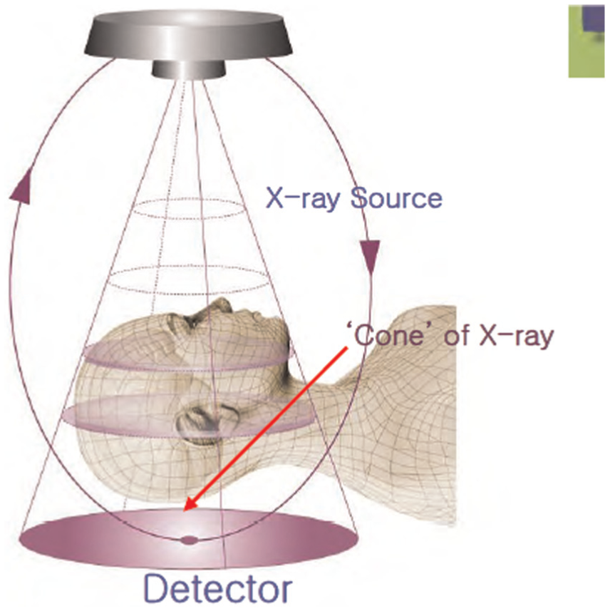
CBCT.
There are many components installed in the CBCT simulator. Therefore, the manufacturing accuracy of each component and assembling accuracy of each module will affect the motion accuracy of this simulator. The errors that come from mechanism manufacturing and assembling will further yield the image shift and that would degrade the quality of 3D image reconstruction. High-accuracy position control was necessary for CBCT machine. 5 In recent years, artificial neural network (ANN) was widely used to solve the optimization problem of science and industry, such as function approximation, pattern recognition, signal processing, and speech recognition. 6 The various types of ANN had been developed and studied for engineering problems because of its powerful capability and functionality. 7
A special class of ANN was the multi-layer feed-forward artificial neural network (FFANN), 8 which was a very popular and efficient tool used to solve a variety of complex problems such as medical image screening, fingerprint identification, and hand-written digit recognition.9,10 One of the most popular supervised training methods for FFANN was backpropagation (BP) learning algorithm, which adjusted the weights in the negative direction of the gradient. 11 And the conjugate gradient (CG) algorithm was following conjugate direction, which generally produced faster convergence than steepest descent direction, to search the solution. 12 Next, Newton’s method involved second derivatives for Hessian matrix of the performance function at the current weights. It spent much time when calculating Hessian matrix. But this method still converged faster than CG algorithm. Then, quasi-Newton’s (QN) method was based on Newton’s method but did not calculate the second derivatives. Instead, an approximate Hessian matrix was updated at each training iteration as a function of the gradient. 13 Therefore, the Levenberg–Marquardt (LM) algorithm was modified by QN method. This algorithm did not compute Hessian matrix second derivatives and used another form of approximation Hessian matrix. 14 LM algorithm was complex but efficient, since not only the gradient but also the Jacobian matrix must be calculated. 15 LM algorithm was a powerful algorithm in improving the convergence speed of the ANN with multi-layer perceptron (MLP) architectures. 16 It was a good combination of Newton’s method and steepest descent. 17 It had not only the convergence speed of Newton’s method but also the convergence capability of steepest descent method. 18 Although LM algorithm had fast convergence speed, it still could not avoid the local minimum problem. 19 One of the problems which occurred during above neural network (NN) training algorithms was overfitting. As a result of this, error in training stage was very small, but the error was large when new data were presented to the network online. To improve the generalization of the NN, the Bayesian regularization modified the performance function into the mean squared errors and the penalty of NN’s weights. 20 The Bayesian regularization assumed the weights and biases of NN is the specific distribution as Bayesian network, combine the LM algorithm with Bayesian regularization could overcome the overfitting problem.8,21
This article proposes a NN corrector to correct the image shift, yielding the degradation of 3D image reconstruction, for each slice captured by CBCT simulator. This NN corrector generates the corrected translation position through one input of the measure data calculated from image shift. The LM learning algorithm adjusts the connected weights and biases of the NN using a supervised gradient descent method, such that the defined error function can be minimized. Bayesian regularization is used to avoid the overfitting and improve the generalized ability of the NN. Finally, the corrected translation n position is fed to be the new position command to verify the image correction performance, and the experimental results verify that the image shift can be reduced by the NN corrector.
CBCT simulator
Hardware of CBCT
The CBCT simulator is composed of three modules: frame, detector, and tube module, as shown in Figure 3. Frame module has one rotational degree-of-freedom (DOF); detector module has one translational DOF; tube module has 2 DOFs which are translation and rotation. The central point of tube module should be aligned with the central point of detector module in the image capturing process to guarantee the accurate image projection.

Three modules of CBCT simulator.
The mode of tomosynthesis
In this article, the CBCT simulator is used to do tomosynthesis, in which detector is fixed and X-ray tube is moved with rotation and translation, as shown in Figure 4. Tomosynthesis mode has the better 2D resolution but the worse 3D resolution after reconstruction comparing to CBCT mode. Although the 3D image quality of tomosynthesis is worse than CBCT, it can get the enough image data for 3D reconstruction without rotating a full circle. Consequently, tomosynthesis not only has the advantage of CBCT but also reduces the radiation dose and exposure cost to get the 2D image from patients. 22
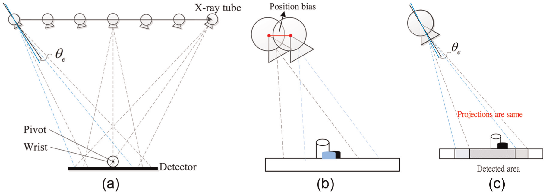
(a) The scan mode of tomosynthesis, (b) translation error affects image shift, and (c) rotation errors do not affect image shift.
In tomosynthesis mode, the motion of the simulator should simultaneously rotate and translate the X-ray tube. Therefore, two errors will be induced in the motion. The translation error will yield the image shift because the object projections in detector are different, as shown in Figure 4(b), where the blue area and the black area are the projections corresponding to positions P1 and P2, respectively. However, even though the rotation error yielded, the object projections still collide together. Figure 4(c) shows rotation error
The image result of CBCT simulator
The coordinate definition of CBCT simulator is shown in Figure 5. Where

The coordinate definition.
In
Theoretically, it is available to calculate the real point


The object projection on detector.
However, the distances for both
Proposed NN image corrector
Since the image shift is nonlinear, a NN image corrector is proposed to correct the image shift to guarantee the accurate image projection. Therefore, the good quality of 3D image reconstruction is acquired.
Architecture of NN corrector
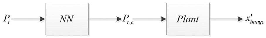
The proposed NN correction system is shown in Figure 7. The target position command

Configuration of the proposed NN correction system.

The transfer functions of image and actual positions.
where
Here, the NN corrector is a single-input and single-output (SISO) system, and it is a two-layer network of four neurons and one neuron corresponding to hidden and output layers, as shown in Figure 9. Then, the neural transfer functions of hidden layer and output layer are tan-sigmoid and linear.

The architecture of proposed NN corrector.
Learning algorithm of NN
Multi-layer NN is always trained by BP algorithm, where the biases and connected weights of the network are adjusted by following the negative direction of the gradient from mean squared error, as shown in Figure 9. The ith input is

and the output of output layer is

Next, the error function is defined as

where

After that the weights and biases are updated as


where k is the iteration,

and the sensitivity of the hidden layer is

LM algorithm, modified Gauss–Newton method, is further used to train the NN in order to improve the convergence rate of defined error function. In Gauss–Newton method, the weights and biases of network are adjusted with the following formulation
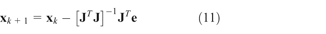
where

And

Then, LM algorithm is defined as

where
In order to avoid the problem of overfitting and improve the generalized ability of the NN, Bayesian regularization is added to the LM learning algorithm. It minimizes a combination of mean squared errors and weights and then determines the correct combination so as to produce a network that generalizes well.
Experimental results
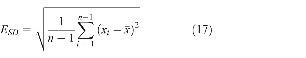
There are two experimental kits used to evaluate the corrected performance of image shift. The first kit is a standard calibration kit with a steel ball in upper layer and ring in lower layer. The second kit is a phantom kit with a matrix of steel balls in both upper and lower layers. Here, the maximum absolute error, mean squared error, and the standard deviation of error are used to measure the corrected performance of image shift


Standard calibration kit
A standard calibration kit with steel ball and ring, as shown in Figure 10(a), is made to measure the image shift. After that the image data scanned by tomosynthesis are used to calculate the shift of steel ball, as shown in Figure 10(b).

(a) The standard kit and (b) projected image.
The proposed NN correction system is shown in Figure 7. The actual position will be different from the target position command since the image shift caused by the mechanism manufacturing and assembling tolerance. In order to improve the image shift, the corrected position obtained using the target position command as the input data of the NN will be the input position command of the CBCT simulator, as shown in Figure 11. There are three sequences of different target position commands applied in the correction experiment. The first sequence of target position commands is 21 points measured by 1° step from −10° to 10°; the second sequence of target position commands is 20 points measured by 1° step from −9.5° to 9.5°; and the third sequence of target position commands is 20 points measured by 1° step from −9.25° to 9.75°. The standard calibration kit is used to do tomosynthesis, and the image data from each point are used to calculate the image shift. The experimental results of image shift with the NN corrector are shown in Figures 12–14 for the above three sequences of target position commands. Additionally, the maximum absolute error and mean squared error of image shift for this experiment are shown in Table 1. The experimental results show the image shift of the standard kit can be reduced from 0.0227 to 0.0012 mm, 0.0237 to 0.00047 mm, and 0.0233 to 0.00028 mm corresponding to the mean squared error of three sequences of different target position commands, and the standard deviation is also reduced from 0.1541 to 0.014 mm, 0.1553 to 0.0117 mm, and 0.1551 to 0.012 mm.
Experimental configuration of proposed NN corrector.

Image shift error with first sequence of target position commands.
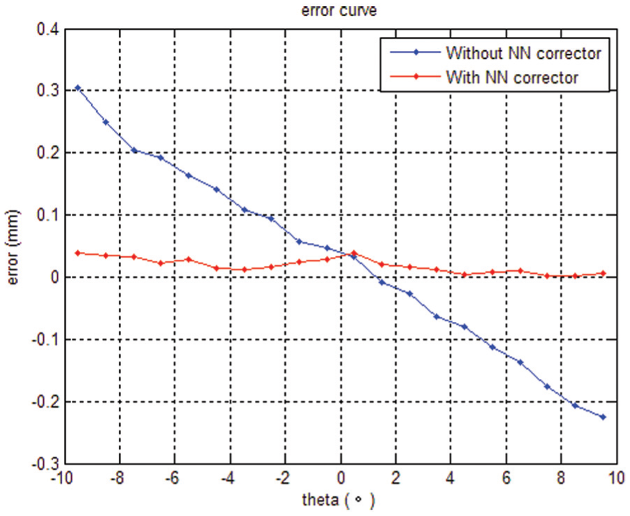
Image shift error with second sequence of target position commands.

Image shift error with third sequence of target position commands.
Image shift error for each sequence of target position commands (mm).

NN: neural network.
We used MATLAB R2012a software to train the NN corrector; the computational time for each training data set is around 3.5 s. Here, the computer platform is Intel i5-4460 CPU with 4GB RAM; the computational speed also proves that our algorithm is available for daily quality assurance.
Phantom calibration kit
In the second case, a phantom calibration kit with two layers of steel balls matrix is made to measure the image shift of multi-points as shown in Figure 15(a). The schematic diagram of the phantom calibration kit, in which the solid circles are in the upper layer and the hollow circles are in the lower layer, is shown in Figure 15(b). Here, nine points of the phantom kit are selected to calculate the image shift, as shown in Figure 16. And the maximum absolute error and mean squared error of each image shift for nine points, which are D4, D5, D6, E4, E5, E6, F4, F5, and F6, are shown in Table 2. In addition, the mean squared error of image shift for upper and lower layers is shown in Tables 3 and 4. The experimental results show the image shift of the phantom kit can be reduced from 0.0103 to 0.00053 mm and 0.00022 to 0.00006 mm corresponding to the mean squared error of upper and lower layers, respectively, and the standard deviation of error is also reduced from 0.1015 to 0.0177 mm and 0.0126 to 0.008 mm.

(a) The phantom kit and (b) the schematic of marker placement in the phantom.
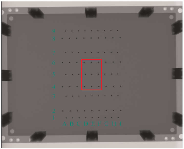
The nine points of the phantom kit (D4, D5, D6, E4, E5, E6, F4, F5, and F6).
Image shift error of each point (mm).

NN: neural network.
Image shift error of upper layer (mm).

NN: neural network.
Image shift error of lower layer (mm).
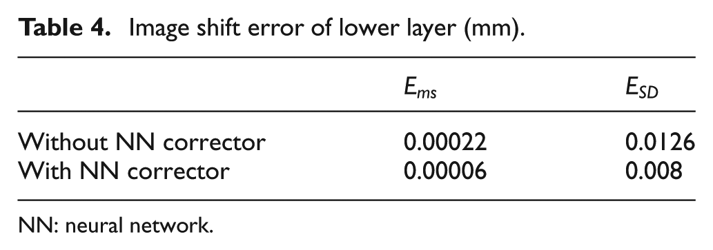
NN: neural network.
Conclusion
This article proposes NN corrector to correct the image shift, yielding the degradation of 3D image reconstruction, in the CBCT simulator. In order to improve the convergence rate and reduce the defined error function, LM algorithm is used to train the NN using the supervised gradient descent method. Moreover, Bayesian regularization is used to avoid the problem of overfitting and improve the generalized ability of the NN. The experimental results show the image shift of the standard kit can be dramatically reduced from 0.0227 to 0.0012 mm, 0.0237 to 0.00047 mm, and 0.0233 to 0.00028 mm corresponding to the mean squared error of three sequences of different target position commands. Additionally, the image shift of the phantom kit can also be reduced from 0.0103 to 0.00053 mm and 0.00022 to 0.00006 mm corresponding to the mean squared error of upper and lower layers, respectively. The experimental results obviously verify that the NN corrector is functional to reduce the image shift effectively.
Footnotes
Acknowledgements
This research was performed with the support of Swissray Asia Healthcare Co., Ltd, Taiwan. The authors particularly thank the Swissray Asia Healthcare Co., Ltd for providing the test samples and for sharing valuable experience of cone-beam computed tomography technology.
Academic Editor: Stephen D Prior
Declaration of conflicting interests
The author(s) declared no potential conflicts of interest with respect to the research, authorship, and/or publication of this article.
Funding
The author(s) received no financial support for the research, authorship, and/or publication of this article.